Machine learning literary genres from 19th century seafaring, horror and western novels

So I got interested in 'digital humanities' and I wanted to try out some of their procedures for doing literary criticism with computers. One basic problem they have is how to classify texts so that, firstly, they can be searched for and found (this is the librarian's problem), but also so that they can be grouped according to content or genre and compared with one another (a literary critic's job). And I realised that the internet is itself a vast text classification and retrieval problem on a scale comparable to the Borgesian infinite library. The Dewey decimal system is simply not going to cut it. I learned that even as I submit these words to this blog, search engine webcrawlers are sucking them all up and throwing them into vast term-document matrices, which they use to match my words to search phrases by calculating cosine similarities and other mathematical measures of correspondence. How to do things with words with machines1. Awesome geek stuff! The problem I've made up for today: train a machine to classify a book into one of three literary genres: Seafaring, Gothic Horror or Western.

Basic document classification methods use the vocabulary of a text to classify it. My expectation is that westerns are saddled with "horses," "trails" and "campfires," whilst nautical tales will loaded with "mainmasts," "captains" and "decks." So, yes, I'm making the naive assumption that a literary genre can be defined by vocabulary. Plainly that's an oversimplification but it isn't *completely* naive, since the superficial elements of subject matter and language *are* very distinct features genres like western & seafaring. Yes, I deliberately picked easy genres :-)

This is a learning exercise so my parameters are:

• Stop and unpack ideas I don't understand; gloss over those I do
• Keep it simple and stick with tools that can easily explain themselves (so, no SVMs or neural nets). I like to be able to lift up the hood and see what is happening inside
• Do everything in Python, even the charts. Please excuse my noob code :-)

Books for the sub-sub machine to read

I've selected a handful of books from each genre. They're mostly 19th century works and as genre pulp-y as I could find.

Seafaring stories

• A Pirate of the Caribbees, by Harry Collingwood
• "Captain Courageous," a Story of the Grand Banks, by Rudyard Kipling
• Mr. Midshipman Easy, by Frederick Marryat
• Narrative of A. Gordon Pym, by Edgar Allan Poe
• Pieces of Eight, by Richard le Gallienne
• Thrilling Narratives of Mutiny, Murder and Piracy, by Anonymous
• Tom Cringle's Log, by Michael Scott

Seafaring adventure stories sound like this:

The white lateen sails of the gun-boat in advance were now plainly distinguishable from the rest, which were all huddled together in her wake. Down she came like a beautiful swan in the water, her sails just filled with the wind, and running about three knots an hour. Mr Sawbridge kept her three masts in one, that they might not be perceived, and winded the boats with their heads the same way, so that they might dash on board of her with a few strokes of the oars. So favourable was the course of the gun-boat, that she stood right between the launch on one bow, and the two cutters on the other; and they were not perceived until they were actually alongside; the resistance was trifling, but some muskets and pistols had been fired, and the alarm was given. -- Mr. Midshipman Easy, by Frederick Marryat

Westerns

• Cattle Brands, by Andy Adams
• Riders of the Purple Sage, by Zane Grey
• Tales of lonely trails, by Zane Grey
• The Trail of the White Mule, by B. M. Bower

Westerns sound like this:

By and by Venters rolled up his blankets and tied them and his meagre pack together, then climbed out to look for his horse. He saw him, presently, a little way off in the sage, and went to fetch him. In that country, where every rider boasted of a fine mount and was eager for a race, where thoroughbreds dotted the wonderful grazing ranges, Venters rode a horse that was sad proof of his misfortunes. -- Riders of the Purple Sage, by Zane Grey

Gothic Horror

• Carmilla, by J. Sheridan LeFanu
• The Fall of the House of Usher, by Edgar Allan Poe
• Famous Modern Ghost Stories, by Various, Edited by Emily Dorothy Scarborough
• Frankenstein, by Mary Wollstonecraft (Godwin) Shelley
• The Damned, by Algernon Blackwood
• The Wendigo, by Algernon Blackwood
• Three Ghost Stories, by Charles Dickens

Gothic Horror stories sound like this:

The wailing assuredly was in my mind alone. But the longer I hesitated, the more difficult became my task, and, gathering up my dressing gown, lest I should trip in the darkness, I passed slowly down the staircase into the hail below. I carried neither candle nor matches; every switch in room and corridor was known to me. The covering of darkness was indeed rather comforting than otherwise, for if it prevented seeing, it also prevented being seen. The heavy pistol, knocking against my thigh as I moved, made me feel I was carrying a child's toy, foolishly. I experienced in every nerve that primitive vast dread which is the thrill of darkness. Merely the child in me was comforted by that pistol. -- The Damned, by Algernon Blackwood

Step 1. Download texts, clean-up & pre-process

The purpose of pre-processing texts is to try and improve the signal-to-noise ratio for the machine learning algorithm. Let's recognise upfront that this is a fairly subjective process. Digital humanities, like any sort of data science or applied statistics, is still as much art as it is science. The modeller will have an intuition or some apriori expectations of the sorts of predictive features they expect will be important and the sorts of confounding noise they should remove.

I like it when data scientists recognise and explain the choices that they make when preprocessing, rather than blindly following a standard method (eg. strip stopwords, stem words, convert to TFIDF form, fit model, profit). Any form of preprocessing designed to improve the signal-to-noise ratio is necessarily eliminating some information deemed irrelevant so that other information is amplified. The risk is that the information eliminated was important. An extreme example: when he does topic modelling, Matthew Jockers uses a POS tagger to elimnate all non-nouns: he details his reasoning in his "secret" recipe post. He makes a good case, I think. For Matthew's inquiries, verbs are 'noise' and contain no useful information. But for lots of other problems, verbs will contain useful information. I certainly expect that there will be certain verbs that are strongly associated with different genres - eg. 'sail' in seafaring, 'ride' in westerns.

Things I'm going to do in this step:

• Download texts from Project Gutenberg
• Strip out Project Gutenberg header & footer
• Strip out all punctuation except full stops
• Create a list of all proper nouns that appear in the text by identifying Mr, Mrs, word pairs in capitals, etc. Use the full stops to differentiate proper nouns from words that are capitalised because they are at the start of a sentence (and so come immediately after a full stop)
• Strip out those proper nouns, and then the full stops
• Create a list of common English "stopwords" to strip out in the next step

I'll be removing ubiquitous, odourless English constructions like "or" and "the" because I don't believe they contain any information useful for classifying genre and, being so common, they can crowd out rarer words. We also strip out all the proper nouns. Proper nouns, such as character names, will quickly be picked up by any sort of model as highly predictive features because they are always specific to a single text. Of course, they're false features because they aren't generalisable to genre.

Things I'm not going to do:

• Use a word stemmer or lemmatizer to convert all tenses of a word to a single form. This can get very messy with older texts, especially where they contain archaic words or colloquialisms (westerns are full of "yuh's")
• Use bigrams, trigrams or ngrams of any sort: let's keep it simple and just use words as independent units
• Use a part-of-speech tagger for anything: there's no need. I want to include all classes of words: verbs, nouns, adjectives, whatever.

# Create reference table of texts, URLs and genre labels
TextArray = [
('Horror','Carmilla','http://www.gutenberg.org/cache/epub/10007/pg10007.txt'),
('Horror','Fall of the House of Usher','http://www.gutenberg.org/files/932/932.txt'),
('Horror','Famous Modern Ghost Stories','http://www.gutenberg.org/cache/epub/15143/pg15143.txt'),
('Horror','Frankenstein','http://www.gutenberg.org/cache/epub/84/pg84.txt'),
('Horror','The Damned','http://www.gutenberg.org/cache/epub/11074/pg11074.txt'),
('Horror','The Wendigo','http://www.gutenberg.org/cache/epub/10897/pg10897.txt'),
('Horror','Three Ghost Stories','http://www.gutenberg.org/files/1289/1289-0.txt'),
('Nautical','A Pirate of the Caribbees','http://www.gutenberg.org/cache/epub/21073/pg21073.txt'),
('Nautical','Captain Courageous','http://www.gutenberg.org/cache/epub/2186/pg2186.txt'),
('Nautical','Mr. Midshipman Easy','http://www.gutenberg.org/cache/epub/6629/pg6629.txt'),
('Nautical','Narrative of Arthur Gordon Pym','http://www.gutenberg.org/ebooks/2149.txt.utf-8'),
('Nautical','Pieces of Eight','http://www.gutenberg.org/cache/epub/17741/pg17741.txt'),
('Nautical','Thrilling Narratives of Mutiny Murder and Piracy','http://www.gutenberg.org/cache/epub/25982/pg25982.txt'),
('Nautical',"Tom Cringle's Log",'http://www.gutenberg.org/cache/epub/7281/pg7281.txt'),
('Western','Cattle Brands (Stories)','http://www.gutenberg.org/cache/epub/12281/pg12281.txt'),
('Western','Riders of the Purple Sage','http://www.gutenberg.org/cache/epub/1300/pg1300.txt'),
('Western','Tales of Lonely Trails','http://www.gutenberg.org/cache/epub/12225/pg12225.txt'),
('Western','The Trail of the White Mule','http://www.gutenberg.org/cache/epub/2063/pg2063.txt')
]
 
# download and import all texts
import urllib2 # the lib that handles the url stuff
GenreCorpus = []
for i,j,k in TextArray:
text = urllib2.urlopen(k).read().replace('n', ' ').replace('r', ' ')
GenreCorpus.append(text)
 
print "Examples from our corpus:"
print "* " + GenreCorpus[1][0:250]
print "* " + GenreCorpus[8][5061:5291]
print "* " + GenreCorpus[15][7039:7230]

Examples from our corpus:

• Project Gutenberg's The Fall of the House of Usher, by Edgar Allan Poe This eBook is for the use of anyone anywhere at no cost and with almost no restrictions whatsoever. You may copy it, give it away or re-use it under the terms of the Project
• "Oh, you're a high-grade machine, with the writing in plain sight," the Philadelphian yawned. "You'll blossom into a credit to your country if you don't take care." "I know it. I'm an American--first, last, and all the time.
• For the first time Jane Withersteen felt Venters's real spirit. She wondered if she would love this splendid youth. Then her emotion cooled to the sobering sense of the issue at stake.

# strip out Gutenberg header & footer
import re
storyStrings = []
for story in GenreCorpus:
textStart = re.search(r'START OF [w]+ PROJECT GUTENBERG EBOOK ["'.ws]+[*]+', story).end()
textEnd = re.search(r'END OF [w]+ PROJECT GUTENBERG EBOOK ["'.ws]+[*]+', story).start()
storyStrings.append(story[textStart:textEnd])
 
# Poe's Narrative of Arthur Gordon Pym doesn't come stand-alone, it's part of a collected works edition.
# We need to trim out of from all the other stories. "Narrative of AGP" is the first story in the connection, followed by "LIGEIA"
# find start of AGP
PymStart = [m.start() for m in re.finditer(r'NARRATIVE OF A. GORDON PYM', storyStrings[10])][1]
# find start of next story in collection ('LIGEIA')
PymEnd = [m.start() for m in re.finditer(r'LIGEIA', storyStrings[10])][1]
storyStrings[10] = storyStrings[10][PymStart:PymEnd]
 
print "[0] Narrative of A. Gordon Pym before cleanup: "
print storyStrings[10][0:200]
 
## clean up text
# Strip out all non-characters EXCEPT full stops - we'll use them to find a list of proper nouns
storyStrings=[re.sub(r'[']', '', text) for text in storyStrings]
storyStrings=[re.sub(r'[^ws.]', ' ', text) for text in storyStrings]
 
print "n[1] Narrative of A. Gordon Pym after stripping punctuation (except full stops): "
print storyStrings[10][0:200]
 
# names and proper nouns
propernouns = []
for story in storyStrings:
propernouns = propernouns + re.findall(r'Mr.[s][w]+', story) # Find all words that start with a capital and appear after "Mr."
propernouns = propernouns + re.findall(r'Mrs.[s][w]+', story)
propernouns = propernouns + re.findall(r'Ms.[s][w]+', story)
propernouns = propernouns + re.findall(r'Miss[s][w]+', story)
# Full names (two words with capital letters) like Harvey Blake. Ensure they come after another word, not a full stop
propernouns = propernouns + [" ".join(word.split()[1:3]) for word in re.findall(r'[s][a-z]+[s][A-Z][a-z]+[s][A-Z][a-z]+[s.]', story)]
# words that start with capital letters and come after another word without a capital letter. like "said Carmilla."
propernouns = propernouns + [word.split()[1] for word in re.findall(r'[a-z]+[s][A-Z][a-z]+[.s]', story)]
 
propernouns = set(propernouns)
print "nNumber of proper nouns: " + str(len(propernouns))
print "nExamples from our list of proper nouns: " + str(sorted(propernouns)[4551:4600])
 
# strip all of these out of the texts
for word in propernouns:
storyStrings = [re.sub(" "+word+" "," ",story) for story in storyStrings]
 
# now remove the full stops and convert everything to lower case
import string
storyStrings = [story.translate(string.maketrans("",""), "_.0123456789").lower() for story in storyStrings]
 
print "n[2] Narrative of A. Gordon Pym after stripping proper nouns & converting to lower case: "
print storyStrings[10][0:200]

[0] Narrative of A. Gordon Pym before cleanup: NARRATIVE OF A. GORDON PYM INTRODUCTORY NOTE UPON my return to the United States a few months ago, after the extraordinary series of adventure in the South Seas and elsewhere, of which an acco

[1] Narrative of A. Gordon Pym after stripping punctuation (except full stops): NARRATIVE OF A. GORDON PYM INTRODUCTORY NOTE UPON my return to the United States a few months ago after the extraordinary series of adventure in the South Seas and elsewhere of which an acco

Number of proper nouns: 7142

Examples from our list of proper nouns: ['Mr. S', 'Mr. Salters', 'Mr. Saunders', 'Mr. Saunderss', 'Mr. Schaefer', 'Mr. Schutz', 'Mr. Seigerman', 'Mr. Seigermans', 'Mr. Shaler', 'Mr. Simpson', 'Mr. Smith', 'Mr. Spaniard', 'Mr. Splinter', 'Mr. Spry', 'Mr. Stains', 'Mr. Sweeneys', 'Mr. Tarry', 'Mr. Thom', 'Mr. Thomas', 'Mr. Tomlinson', 'Mr. Troop', 'Mr. Trounce', 'Mr. William', 'Mrs', 'Mrs Easy', 'Mrs Trunnions', 'Mrs C', 'Mrs Campana', 'Mrs Easy', 'Mrs Easy.', 'Mrs Easys', 'Mrs Hogg', 'Mrs Job', 'Mrs Mangrove', 'Mrs Mangrove.', 'Mrs Oxbelly', 'Mrs Oxbellys', 'Mrs Palma', 'Mrs Palmas', 'Mrs Peter', 'Mrs Potiphart', 'Mrs.', 'Mrs. Borlsover', 'Mrs. Brigham', 'Mrs. Brighams', 'Mrs. Bryer', 'Mrs. Casey', 'Mrs. Cheyne', 'Mrs. Cheynes']

[2] Narrative of A. Gordon Pym after stripping proper nouns & converting to lower case:

narrative of a gordon pym introductory note upon my return to the a few months ago after the extraordinary series of adventure in the and elsewhere of which an account is given in the follow

# Prepare list of stopwords
stopfile = urllib2.urlopen('http://ir.dcs.gla.ac.uk/resources/linguistic_utils/stop_words')
stopwords = stopfile.read().replace('n', ' ').replace('r', ' ').lower().split()
# add a handful more
stopwords = stopwords + ['said','chapter']
# this is what the list looks like
print "Examples of stopwords: " + str(stopwords[110:120])

Examples of stopwords: ['give', 'go', 'had', 'has', 'hasnt', 'have', 'he', 'hence', 'her', 'here']

Step 2. Convert text data to vector space, understand what that means

The simplest sort of "vector space" is a big table with documents as rows, words as columns, and the frequency that those words appear at each intersection. It's sometimes referred to as the "bag of words," since we're throwing away all context and just counting how often words appear in documents.

Steps:

• Convert corpus to bag-of-words format & strip out stopwords
• Try Euclidean and Cosine similarity measures to see which texts are more or less like others
• Do some visualisations

# Before we do transformations, for sake of convenience let's make a few lists of labels
genrelabels = [i for i,j,k in TextArray]
genres = set(genrelabels)
textlabels = [j for i,j,k in TextArray]
 
# transform corpus into vector space
from sklearn.feature_extraction.text import CountVectorizer
cv = CountVectorizer(stop_words = stopwords)
stories_tdm = cv.fit_transform(storyStrings).toarray()
 
# Examine term-document matrix
import numpy as np
print "Term-document matrix contains %d books and %d features (vocab)." %(stories_tdm.shape[0], stories_tdm.shape[1])
vocab = np.array(cv.get_feature_names())
print "n Examples from features (vocab): " + str(vocab[10000:10030])

Term-document matrix contains 18 books and 30682 features (vocab).

Examples from features (vocab): [u'fight' u'fighter' u'fighters' u'fightez' u'fightin' u'fighting' u'fights' u'figments' u'figs' u'figurantes' u'figure' u'figured' u'figurehead' u'figures' u'figurin' u'figuring' u'filamentous' u'filaments' u'filbert' u'filberts' u'file' u'filed' u'files' u'filial' u'filing' u'filled' u'filling' u'fillip' u'fills' u'film']

The vocab includes words that appear many times in different tenses, for example, "need," "needed", "needing," and "needful." All those words have the common root of "need" and this is where we could use a word stemmer/lemmatizer to try and convert them all to that common form. Arguably this would improve the signal-to-noise ratio, since we'd collapse various sparse features into a single, stronger feature. That said, I'm not going to do it because word stemmers are still fairly rough and the results are often quite messy, especially where you have novels that include archaic terms or phonetically-written dialogue (as you tend to get in westerns, for example).

# convert to a convenient pandas dataframe form
import pandas
# Make an array of both genre & title to act as hierarchical index in pandas
titleindex = [[i for i,j,k in TextArray],[j for i,j,k in TextArray]]
# Convert TDM into pandas DF
stories_tdm_df = pandas.DataFrame(data=stories_tdm, index=titleindex, columns=vocab)
 
# For example:
print "Raw example of term-document matrix:"
print stories_tdm_df[['night','sail','horse','did','man','time']]

Raw example of term-document matrix:

night sail horse did man time

Carmilla 42 0 4 62 16 64

Fall of the House of Usher 6 0 2 8 2 4

Famous Modern Ghost Stories 145 0 12 156 124 155

Frankenstein 88 5 0 119 129 97

Pieces of Eight 67 13 1 80 119 99

The Trail of the White Mule 51 0 2 117 166 88

<...>

Quantifying texts allows us to ask questions about them in mathematical ways. Take the question, "Which texts are similar?" There's a number of mathematical ways of asking that question, the two most common being Euclidean distance and cosine similarity.

Euclidean distance: Imagine each book as a single point in our 30,682-dimensional vector space. The closer two points are together, the most similar they are.

Cosine similarity: Each book is a vector (in the physics sense, not the computer science sense) starting from the origin and with a direction defined by it's 30,682 features. The smaller the angle between two vectors = the more similar the texts. (There's a clear discussion of the formula here).

Let's try both. For visualisations, we obviously can't do plots in 30,682 dimensions, so I'll just show two: "man" and "time." You'll have to imagine the other 30,680 dimensions :-)

# Calculate similarity matrix using Euclidean distance
from sklearn.metrics import pairwise_distances
from scipy.spatial.distance import cosine
dist_out = 1-pairwise_distances(stories_tdm_df, metric="Euclidean")
 
# create a plot space for two plots
fig, ax = plt.subplots(1,2,figsize=(14,5))
## scatterplot of texts on 2D vector space
# plot points, coloured by genre. Must add them to plot one by one to get the cursed matplotlib legend to work
for gen,colour in zip(genres,('blue','green','red')):
ax[0].scatter(stories_tdm_df['man'].ix[gen],stories_tdm_df['time'].ix[gen],c=colour,label=gen,s=100)
ax[0].set_xlabel("# occurrences 'man'")
ax[0].set_ylabel("# occurrences 'time'")
ax[0].set_title("TDM frequency scatterplot (2D)")
ax[0].legend(loc=4)
# label an outlier
ax[0].annotate(
"Tom Cringle's Log",
xy = (stories_tdm_df['man'].ix[("Nautical","Tom Cringle's Log")]-10, stories_tdm_df['time'].ix[("Nautical","Tom Cringle's Log")]), xytext = (-30, 20),
textcoords = 'offset points', ha = 'center', va = 'bottom',
bbox = dict(boxstyle = 'round,pad=0.5', fc = 'yellow', alpha = 0.5),
arrowprops = dict(arrowstyle = '->', connectionstyle = 'arc3,rad=0.4',color='black'))
 
## heatmap of Euclidean distance
column_labels = list(stories_tdm_df.index)
row_labels = list(stories_tdm_df.index)
data = np.array(dist_out)
ax[1].pcolor(data, cmap=plt.cm.Reds)
ax[1].set_xticks(np.arange(data.shape[1])+0.5, minor=False)
ax[1].set_yticks(np.arange(data.shape[0])+0.5, minor=False)
ax[1].invert_yaxis()
ax[1].yaxis.tick_right()
ax[1].set_xticklabels(row_labels, minor=False,rotation=90)
ax[1].set_yticklabels(column_labels, minor=False)
ax[1].set_title("Heatmap of Euclidean similarities");

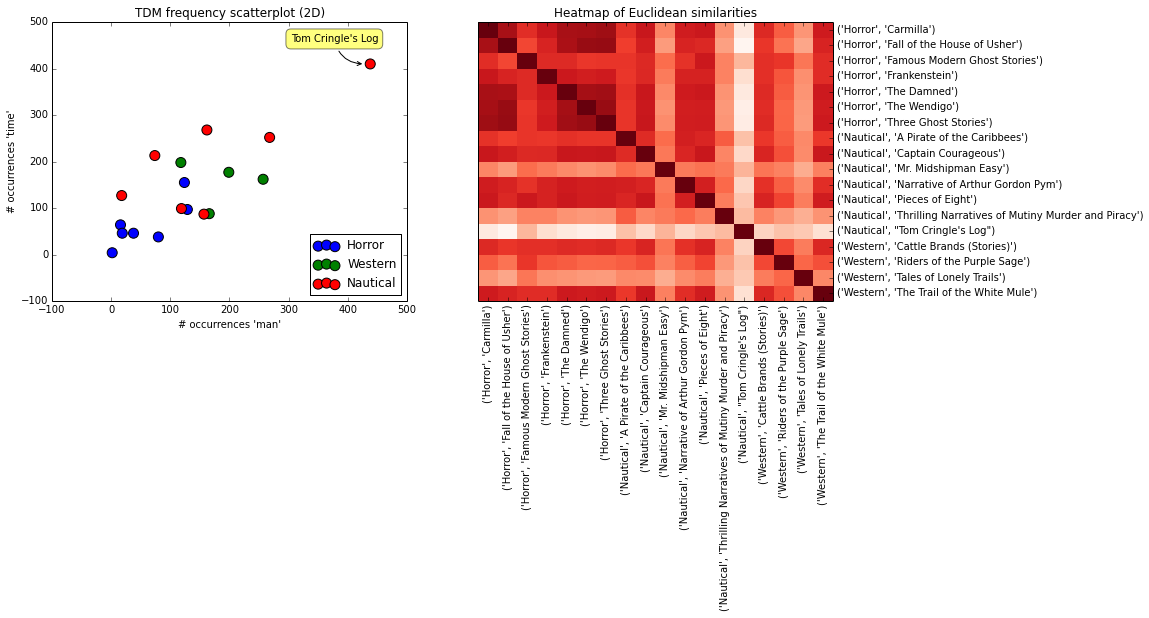
Doesn't work so well. It's because distances between books are more a function of the length of the book (and thus how often words can appear), rather than the composition of words. Hence why Tom Cringle's Cabin is especially dissimilar from all the other texts: because it is so long. At 240k words, it is twice as long as the next longest in my corpus. For that reason, it contains much higher frequencies of all those common words like "man" and "time."

We might get a better result if we converted our data into words as a proportion of each text:

# Convert df into proportions
tdm_percent = stories_tdm_df.apply(np.float32).apply(lambda x: x/x.sum(axis=1),axis=1)
# calculate Euclidean similarity matrix again
dist_out = 1-pairwise_distances(tdm_percent, metric="Euclidean")
 
# create a plot space for two plots
fig, ax = plt.subplots(1,2,figsize=(14,5))
## scatterplot of texts on 2D vector space
# plot points, coloured by genre. Must add them to plot one by one to get the cursed matplotlib legend to work
for gen,colour in zip(genres,('blue','green','red')):
ax[0].scatter(tdm_percent['man'].ix[gen],tdm_percent['time'].ix[gen],c=colour,label=gen,s=100)
ax[0].set_xlabel("# occurrences 'man'")
ax[0].set_ylabel("# occurrences 'time'")
ax[0].set_title("TDM proportion scatterplot (2D)")
ax[0].legend(loc=4)
# label an outlier
ax[0].annotate(
"Tom Cringle's Log",
xy = (tdm_percent['man'].ix[("Nautical","Tom Cringle's Log")], tdm_percent['time'].ix[("Nautical","Tom Cringle's Log")]), xytext = (30, -70),
textcoords = 'offset points', ha = 'center', va = 'bottom',
bbox = dict(boxstyle = 'round,pad=0.5', fc = 'yellow', alpha = 0.5),
arrowprops = dict(arrowstyle = '->', connectionstyle = 'arc3,rad=0.4',color='black'))
 
## heatmap of Euclidean distance
column_labels = list(tdm_percent.index)
row_labels = list(tdm_percent.index)
data = np.array(dist_out)
ax[1].pcolor(data, cmap=plt.cm.Reds)
ax[1].set_xticks(np.arange(data.shape[1])+0.5, minor=False)
ax[1].set_yticks(np.arange(data.shape[0])+0.5, minor=False)
ax[1].invert_yaxis()
ax[1].yaxis.tick_right()
ax[1].set_xticklabels(row_labels, minor=False,rotation=90)
ax[1].set_yticklabels(column_labels, minor=False)
ax[1].set_title("Heatmap of Euclidean similarities using proportions");

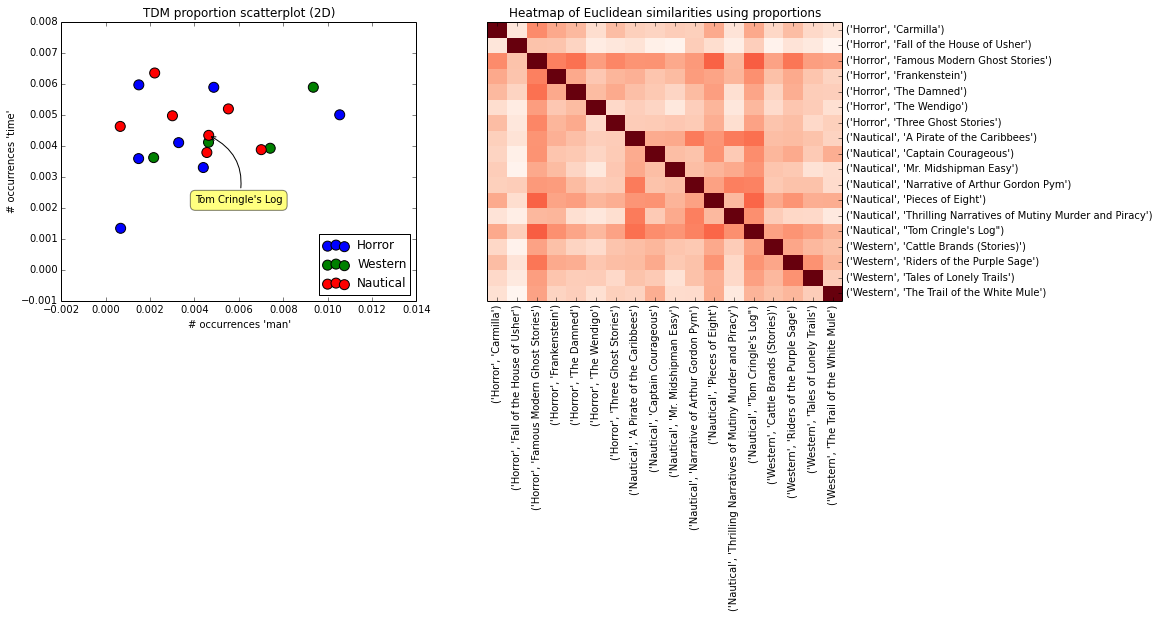
This is better, but not all that promising for our venture. What I'd like to see on the heatmap is dark red rectangles where books intersect with other books from the same genre, and white space where they intersect with books from other genres. But Euclidean measures of similarity are showing more of a patchwork, without clear relationships between genres. Let's try using cosine similarity:

# Calculate similarity matrix using cosine similarity
from sklearn.metrics import pairwise_distances
from scipy.spatial.distance import cosine
dist_out = 1-pairwise_distances(stories_tdm_df, metric="cosine")
 
# Calculate distance matrix using cosine similarity
from sklearn.metrics import pairwise_distances
from scipy.spatial.distance import cosine
dist_out = 1-pairwise_distances(stories_tdm_df, metric="cosine")
 
# create a plot space for two plots
fig, ax = plt.subplots(1,2,figsize=(14,5))
## scatterplot of texts as vectors. all start at (0,0)
origin=np.zeros((1, 18))
colour = pandas.Categorical(genrelabels).labels
ax[0].quiver(origin,origin,list(stories_tdm_df['saw']),list(stories_tdm_df['know']), colour, cmap=plt.cm.brg, scale_units='xy', angles='xy', scale=1)
ax[0].axis([0, 300, 0, 200])
ax[0].set_xlabel("# occurrences 'saw'")
ax[0].set_ylabel("# occurrences 'know'")
ax[0].set_title("TDM vector plot (2D)")
# label some texts
ax[0].annotate(
"Tom Cringle's Log",
xy = (stories_tdm_df['saw'].ix[("Nautical","Tom Cringle's Log")], stories_tdm_df['know'].ix[("Nautical","Tom Cringle's Log")]), xytext = (90, -10),
textcoords = 'offset points', ha = 'center', va = 'bottom',
bbox = dict(boxstyle = 'round,pad=0.5', fc = 'yellow', alpha = 0.5),
arrowprops = dict(arrowstyle = '->', connectionstyle = 'arc3,rad=0.4',color='black'))
ax[0].annotate(
"Famous Modern Ghost Stories",
xy = (stories_tdm_df['saw'].ix[("Horror","Famous Modern Ghost Stories")], stories_tdm_df['know'].ix[("Horror","Famous Modern Ghost Stories")]), xytext = (-50, 20),
textcoords = 'offset points', ha = 'center', va = 'bottom',
bbox = dict(boxstyle = 'round,pad=0.5', fc = 'yellow', alpha = 0.5),
arrowprops = dict(arrowstyle = '->', connectionstyle = 'arc3,rad=0.4',color='black'))
ax[0].annotate(
"Pieces of Eight",
xy = (stories_tdm_df['saw'].ix[("Nautical","Pieces of Eight")], stories_tdm_df['know'].ix[("Nautical","Pieces of Eight")]), xytext = (90, -10),
textcoords = 'offset points', ha = 'center', va = 'bottom',
bbox = dict(boxstyle = 'round,pad=0.5', fc = 'yellow', alpha = 0.5),
arrowprops = dict(arrowstyle = '->', connectionstyle = 'arc3,rad=0.4',color='black'))
 
## heatmap of Cosine similarities
column_labels = list(stories_tdm_df.index)
row_labels = list(stories_tdm_df.index)
data = np.array(dist_out)
ax[1].pcolor(data, cmap=plt.cm.Reds)
ax[1].set_xticks(np.arange(data.shape[1])+0.5, minor=False)
ax[1].set_yticks(np.arange(data.shape[0])+0.5, minor=False)
ax[1].invert_yaxis()
ax[1].yaxis.tick_right()
ax[1].set_xticklabels(row_labels, minor=False,rotation=90)
ax[1].set_yticklabels(column_labels, minor=False)
ax[1].set_title("Heatmap of cosine similarities");

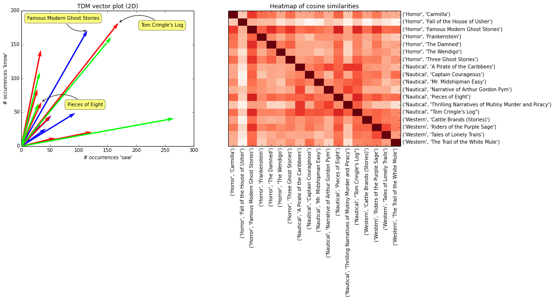
Cosine similarity returns a different picture. Take a look at Famous Modern Ghost Stories. Using Cosine similarity, it is judged to be more similar to Pieces of Eight than to Tom Cringle's Log. Though Famous Modern and Tom Cringle contain similar absolute numbers of words (like "saw" and "know"), by proportion it is more similar to Pieces of Eight, and hence the angle between the two vectors is smaller. If you scroll back up to our first heat map of similarities using Euclidean distance, you'd see that Famous Modern and Tom Cringle are found to be very dissimilar.

The overall results are better than the previous two measures of similarity, but not much. It's barely more promising than the proportional Euclidean distance results. A faint but visible rectangle of red can be seen on the heat map where the nautical novels intersect, but there's little evidence of similarity between the other genres' texts.

Neither method of measuring similarity is telling me what I want to hear: that our genres are internally homogeneous and externally heterogeneous in terms of vocabulary. But that doesn't mean we should give up. For two reasons I don't trust these similarity measures to be conclusive evidence that our task is futile:

1. They are very blunt: they compare texts across the entire ~31k dimensions of vector space. I'm expecting that there is a handful of vocabulary from each genre which will be strongly discriminative, with the remaining ~30k words merely noise. A Euclidean distance measure will be mostly determined by those 30k irrelevant words.
2. Both methods have their shortcomings: Euclidean distance is influenced by the magnitude of features (words) and risks grouping texts as similar based on their length. A short western story and a short seafaring story will be more similar to each other than they would to long western or seafaring novels: they would both contain similar frequencies of common words like "man" and "time," etc. Conversely, cosine similarity has the opposite drawback. By measuring the angle between vectors it is intentionally designed to abstract away the magnitude of features. Cosine similarity takes no account of magnitude at all, so we can find that a short horror text with the odd sailing word is more similar to nautical novels than other horror novels.

An ideal measure of similarity would want to strike a balance between the two approaches. The literature suggests a few more sophisticated measures of similarity such as Jacard's index, but we're going to move on and try a different approach. So, let's leave measures of similarity behind and look instead for specific vocabulary belonging to each genre.

Step 3. Look for discriminative words

How to find the words which are especially representative of each genre? In my mind, I'm expecting words like "topsail" and "mizzenmast" from the seafaring novels, and "blood" and "fear" from the horror novels.

Steps:

• Look at most frequent words in each genre
• Use Mann-Whitney test to identify most discriminative words in each genre

# top words by genre
k_feature_genre=stories_tdm_df.groupby(level=0).sum() # sum across genres
df=k_feature_genre.T
for genre in genres:
df.sort(columns=genre,ascending=False,inplace=True)
print "nMost common words in " + genre + " genre: " + (", ".join([i for i in list(df[genre].head(10).index)]))
 
# visualise some of these common words in a heat map
commonwords = ['did', 'like', 'time', 'man', 'little', 'eyes', 'night', 'came', 'saw', 'know', 'water', 'boat', 'ship']
 
fig, ax = plt.subplots(1,1,figsize=(7,5))
column_labels = list(stories_tdm_df[commonwords].index)
row_labels = commonwords
data = np.array(stories_tdm_df[commonwords])
ax.pcolor(data, cmap=plt.cm.Reds)
ax.set_xticks(np.arange(data.shape[1])+0.5, minor=False)
ax.set_yticks(np.arange(data.shape[0])+0.5, minor=False)
ax.invert_yaxis()
ax.yaxis.tick_right()
ax.set_xticklabels(row_labels, minor=False,rotation=90)
ax.set_yticklabels(column_labels, minor=False)
ax.set_title("Heatmap of # of common words in texts");

Most common words in Horror genre: did, like, time, man, little, eyes, night, came, saw, know

Most common words in Western genre: man, did, like, time, little, long, got, saw, came, men

Most common words in Nautical genre: time, like, little, water, man, men, sea, boat, ship, long

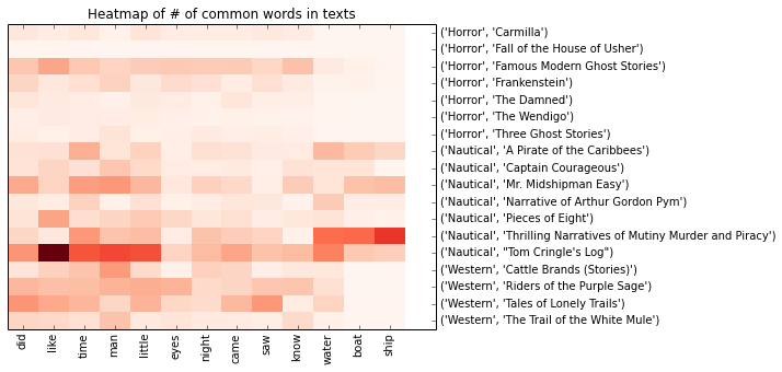
Despite earlier stripping out stopwords, most of these common words are still odourless, functional things. There's a few evocative words in here: "water," "boat" & "ship" in Nautical; "night" in Horror. But, for the most part, this is not the sort of colourful vocab we'd expect to define these genres. More importantly, these words aren't very discriminative. The heat map shows that most of the words are well-represented across all genres. Notable exceptions are "boat" and "ship" which appear to be almost exclusively confined to the nautical texts.

A better way to identify discriminative words would be to use a statistical test like the Mann-Whitney U. The application of the Mann-Whitney test to a tiny corpus like this is a little questionable... But I want to do it anyway after reading Ted Underwood's convincing demonstration of it. (For those who aren't familiar with the test, there's a nice illustration of how it works here).

For each word I'll be doing three tests. In each test, I compare the texts of one genre with the texts of the other two. Again, in a slightly lazy fashion, I'm going to ignore the significance results of the test. I'm sort of expecting that, with such a small corpus, we'll have lots of non-signicant results. What I really want is a measure of the discriminatory effect size of each word so we can rank them. So, we'll take the U statistic as a measure of power, but we'll make an adjustment to account for variations in sample sizes by calculating U/(n1 × n2) (where n1 & n2 are the sample sizes of the two groups). (For those interested, there's a discussion here. The Mann-Whitney doesn't capture the direction of the effect, but I'll assign it by comparing the median # of times that a word is used in texts.

## IDENTIFY MOST DISCRIMINATIVE WORDS
from scipy import stats
# create a quick list of column names for each genre
colnames = stories_tdm_df.index
horrorcols = colnames[0:7]
nauticalcols = colnames[7:14]
westerncols = colnames[14:18]
 
# define function to calculate discriminative effect size from U
def discrimpower(books1, books2):
a = stats.mannwhitneyu(books1, books2)[0] # calculate Mann-Whitney U significance level
b = a / (books1.count() * books2.count() ) # adjust U for sample-size
if books1.median() > books2.median(): # capture the 'direction' of the effect - which side is over-represented
return b
return -b
 
# calculate discrim power values for every word 3 times. For each word, compare each genre's texts against texts from the other two
words_tdm = stories_tdm_df.T
words_tdm['MWU_Horror'] = words_tdm.apply(lambda row: discrimpower(row[horrorcols], row[colnames - horrorcols]),axis=1)
words_tdm['MWU_Nautical'] = words_tdm.apply(lambda row: discrimpower(row[nauticalcols], row[colnames - nauticalcols]),axis=1)
words_tdm['MWU_Western'] = words_tdm.apply(lambda row: discrimpower(row[westerncols], row[colnames - westerncols]),axis=1)
 
# Pull out lowest MWUs for each genre. Note that this is convoluted for a good reason:
# The U scores get small enough for Python float to round them to 0.0, but Python retains the sign.
# ie. we have scores of +0.0 and -0.0!
# DataFrame.sort doesn't distinguish between -0.0 and +0.0, so -0.0's will be returned as smallest value >0
# Therefore, we must use the math.copysign function to retrieve the sign and ensure we get the smallest values >= +0.0
print "Most overrepresented words in Westerns stories are: " + str(", ".join(list(sort(words_tdm[words_tdm.apply(lambda x: math.copysign(1,x['MWU_Western'])>0,axis=1)]['MWU_Western']).head(30).index)))
print "nMost overrepresented words in Seafaring stories are: " + str(", ".join(list(sort(words_tdm[words_tdm.apply(lambda x: math.copysign(1,x['MWU_Nautical'])>0,axis=1)]['MWU_Nautical']).head(30).index)))
print "nMost overrepresented words in Horror stories are: " + str(", ".join(list(sort(words_tdm[words_tdm.apply(lambda x: math.copysign(1,x['MWU_Horror'])>0,axis=1)]['MWU_Horror']).head(30).index)))
 
## VISUALISE 5 words from each on heat map
# Many of these highly-discriminative words occur relatively rarely, so there's no point looking at a simple frequency heatmap
# To make the penetrations stand out, we'll convert counts into percentages across the corpus of stories
bestwords = ["coyote", "outlaws", "trigger", "bluntly", "corral", "tiller", "galley", "hoisted", "hatchway", "sharks", "analysis", "superstition", "sentences", "inexplicable", "mysteries"]
column_labels = list(stories_tdm_df[bestwords].index)
row_labels = bestwords
# calculate percentage distribution for each word
tdm_percent = stories_tdm_df.apply(np.float32).apply(lambda x: x/x.sum(axis=1),axis=1)
data = array(tdm_percent[bestwords])
 
fig, ax = plt.subplots(1,1,figsize=(7,5))
ax.pcolor(data, cmap=plt.cm.Reds)
ax.set_xticks(np.arange(data.shape[1])+0.5, minor=False)
ax.set_yticks(np.arange(data.shape[0])+0.5, minor=False)
ax.invert_yaxis()
ax.yaxis.tick_right()
ax.set_xticklabels(row_labels, minor=False,rotation=90)
ax.set_yticklabels(column_labels, minor=False)
ax.set_title("Heatmap of proportion of selected highly discriminatory words as identified by Mann-Whitney U test");

Most overrepresented words in Westerns stories are: hell, outlaws, trigger, bluntly, outfit, wanted, coyote, drive, corral, organized, trail, throwed, grove, trails, halted, camp, pack, slope, reckon, game, needed, browned, jawed, shoot, herd, snorted, groves, slowed, worried, headed

Most overrepresented words in Seafaring stories are: tiller, sail, boat, galley, hoisted, sails, sharks, shark, lee, anchor, sea, deck, beam, crew, hatchway, anchors, rum, masts, decks, lashed, reef, gunwale, keel, starboard, port, aft, ships, cruise, jib, mainsail

Most overrepresented words in Horror stories are: analysis, superstition, sentences, inexplicable, unnatural, undisturbed, mysteries, landscape, vital, haunted, passionate, abhorrence, downstairs, afflicted, include, hysteria, confessing, nervousness, influenced, autumn, nightmare, notes, shiver, terror, coincidence, childish, bedroom, oppressed, tumultuous, younger

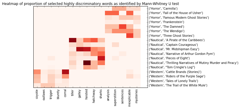
That's the kind of vocab I was hoping to find! Evocative words like "outlaw" and "coyote" from the westerns, "hoisted" and "rum" from the nautical stories, and "unnatural" and "haunted" from horror. And the heatmap shows how these words are strongly confined to a single genre.

I think that horror is slightly less convincing than the other two genres. Some of the words, such as "sentences" and "analysis," don't strike me as evocative of gothic horror. The heat map shows that some of the most discriminative words from horror aren't exclusively confined to those texts. They turn up in other texts, just less often. My hypothesis would be that, compared to the western & seafaring genres, horror is less homogeneous. Seafaring novels will always contain lots of sailing terms; Western novels will always contain horses and trails; but Horror novels are sometimes in haunted houses, sometimes in old castles. Sometimes they include vampires, sometimes ghosts. That which defines gothic horror as a genre is less on the surface, less superficial. That said, there is a lot of anxious, introspective monologues and contemplation of dark forces under the bed - so we do get descriptive words like "mysteries" and "nervousness" coming through.

Many of these words are very uncommon. Some of the most spectacularly predictive words appear only in a single genre. For example, "outlaws." This makes somewhat of a mockery of the Mann-Whitney test but it's still a true result. A word that only appears in Westerns is a very discriminative word. For example:

print stories_tdm_df[['outlaws','tiller','analysis']]

outlaws tiller analysis

Famous Modern Ghost Stories 0 0 3

Frankenstein 0 0 1

Nautical A Pirate of the Caribbees 0 20 0

Pieces of Eight 0 2 0

Tales of Lonely Trails 1 0 0

The Trail of the White Mule 3 0 0

<...>

Before we move on to building the classification model, let's just pick a couple of oddest words and see how they appear in context. I'm curious to know how "analysis" and "sentences" turn up in horror novels. To do this, the NLTK package provides a quick, easy way to do this with its concordance() function.

# Convert horror texts into NLTK.Text format and merge them together into one big Text
import nltk
horror_nltk = [nltk.Text(nltk.word_tokenize(" ".join([story for story in storyStrings[0:7]])))]
 
# Show contexts in which "analysis" is used
print "Concordance view of the word 'analysis' in horror texts:"
print horror_nltk[0].concordance('analysis', width=120)
 
# Show contexts in which "setences" is used
print "nConcordance view of the word 'sentences' in horror texts:"
print horror_nltk[0].concordance('sentences', width=120)

Concordance view of the word 'analysis' in horror texts:Building index... `Displaying 8 of 8 matches:

• cts which have the power of thus affecting us still the analysis of this power lies among considerations beyond our dept
• ntensity an epic sweep unknown in actuality in the last analysis man is as great as his daydreams or his nightmares ghos
• ever though it refused to yield its meaning entirely to analysis did not at the time trouble me by passing into menace y
• his i realized what he realized only with less power of analysis than his was on the tip of my tongue to tell him at las
• an eternal hell imagination was vivid yet my powers of analysis and application were intense by the union of these qual
• rp impression is alone of value in such a case for once analysis begins the imagination constructs all kinds of false in
• n i adopted neither course reflection certainly without analysis of what was best to do for my sister myself or i took u
• fugitive emotion otherwise escaped his usually so keen analysis d fago he was vaguely aware might cause trouble somehow

Concordance view of the word 'sentences' in horror texts: Displaying 15 of 15 matches:

• on the possible meanings of the violent and incoherent sentences which i had just been reading we had nearly a mile to
• hild is fatigued let her be seated and i will in a few sentences close my dreadful story squared block of wood which la
• climax and tried to ignore or laugh at the occasional sentences he flung into the emptiness of these sentences moreove
• asional sentences he flung into the emptiness of these sentences moreover were confoundedly disquieting to me coming as
• totally different point of view composed such curious sentences and hurled them at me in such an inconsequential sort
• ows of capital letters short words long words complete sentences copy book tags whole thing in fact had the appearance
• a on the other side of the bed curtain he saw the last sentences that had been written its too late he read friends alr
• nt to go and hear that little conceited fellow deliver sentences out of a pulpit i recollected what he had said of m wa
• e haze along that depressing that aped a riverbank and sentences from the letter flashed before my eyes and stung me pi
• ing on the writers mind and i felt uneasy studying the sentences brought however no revelation but increased confusion
• bout the place and i had taken it for one of her banal sentences and paid no further attention i realized now that it w
• rst vehemently forth again had hidden between her calm sentences as it had hidden between the lines of her letter swept
• here repeated it in her eyes and gestures and laconic sentences lay the conviction of great beating issues and of mena
• nted night passed over the lonely camp crying startled sentences and fragments of sentences into the folds of his blank
• lonely camp crying startled sentences and fragments of sentences into the folds of his blanket a quantity of gibberish

Hmm. Although both words are fairly unique to our horror genre texts, neither one is used in a consistent way. The word 'sentences' turns up a couple of times in reference to reading a book/letter/diary, a couple of times referring to somebody talking or preaching, and once in the classic way that you find in Poe - with the author referring to the document he is writing ("I will in a few sentences close my dreadful story..."). It's not clear to me why either of these words should be particularly associated with horror. I suspect it is simply relative to the other two genres. It could also be simple statistical noise - both words are rare, even in the horror texts.

Step 4. Develop simple model for classifying a text into genre

The Mann-Whitney test identified words that were typically both uncommon and confined to a single genre. They were very powerful discriminators and I can imagine doing a pretty good job of classifying stories with just a handful of them. I'd hazard a guess that a rule of thumb like, "If you see the words 'trail' and 'cowboy' then you're reading a western," would perform amazingly well. (Yes, that's mostly a function of the easy genres I've selected...)

A simple model is very appealing, but it ignores a lot of the information available. I'm curious to see if we can develop a more complex model which uses all the information we have available in the ~31k words in our corpus. Not just those words which are highly specific to one genre, but also words that have slight probabilistic biases towards a genre.

• Convert to texts to TFIDF representation to boost strength of infrequent but discriminative words
• Fit multinomial naive Bayes classification model
• Score some texts - Dracula, Moby Dick & The Virginian: A Horseman of the Plains
• Examine how it works

TFIDF weighted vector space

The problem we've seen is that really common words aren't very useful for discrimination, but they dominate over the very discriminatory rare words. So we implement what's called TFIDF ("term frequency - inverse document frequency") weighting. In TFIDF-weighted vector space, a weighting is applied so that words which occur in fewer documents are strengthened relative to words which appear in lots of documents. The purpose is, once again, to try to improve the signal-to-noise ratio. We've seen how the most discriminative words tend to be relatively uncommon ones that are localised to documents of a single genre. Conversely, words that are poorly discriminative tend to be ones that appear in all texts - for example, "man" and "time." The purpose of TFIDF is to boost the weight of the former type of word.

The formula is: # of times word appears in document / # of documents where word appears at least once

The next code output shows how both "night" and "sail" appear in standard TDM form and then TFIDF weighting. You'll see that "sail," which appears in roughly half as many texts, doubles its weighting relative to "night." Look at "A Pirate of the Caribees."

# create TFIDF
from sklearn.feature_extraction.text import TfidfTransformer
transformer = TfidfTransformer()
stories_tfidf = transformer.fit_transform(stories_tdm)
# load into pandas DF
stories_tfidf_df = pandas.DataFrame(data=stories_tfidf.toarray(), index=titleindex, columns=vocab)
 
# Unweighted scores
print "Simple TDM frequencies:n"
print stories_tdm_df[['night','sail']]
 
# TFIDF scores
print "nnAfter TFIDF transformation:n"
print stories_tfidf_df[['night','sail']]

Simple TDM frequencies:

night sail

• Carmilla 42 0
• Frankenstein 88 5
• Captain Courageous 41 14
• Pieces of Eight 67 13
• Tom Cringle's Log 182 139
• Tales of Lonely Trails 101 0

After TFIDF transformation:

night sail

• Carmilla 0.099224 0.000000
• Frankenstein 0.096519 0.009582
• Captain Courageous 0.042575 0.025401
• Pieces of Eight 0.074244 0.025169
• Tom Cringle's Log 0.063533 0.084780
• Tales of Lonely Trails 0.043073 0.000000

(This is far from the perfect solution. Although it is better than nothing, there will be uncommon but discriminative words which will not benefit from the TFIDF weighting. TFIDF only boosts uncommon words if they appear in relatively few documents. It does nothing for words that are very common in one genre but still appear occassionally in every other document. Take the example of the word "hell." "Hell" is a dstinctive word which occurs disproportionately often in Westerns, but it doesn't benefit much from the TFIDF weighting because it still appears once or twice in most of our other texts.)

Multinomial Naive Bayesian Classification

Now that we've given a bit more weight to those less common but discriminative words, let's fit a classification model. I'm going to use multinomial naive Bayes. There are alternatives: multinomial linear regression (probably not so good given the distribution of words is very non-parametric with lots of 0's), support vector machines (currently very popular for text classification problems but too opaque for this exercise), neural networks & random forests (ditto - they work well, but painful to figure out how they are making classifications)... MNBC is simple and easy to dissect, so we can examine which words are making the largest contributions.

In plain English, the naive Bayes classifier learns how likely it is to find each individual word in each different genre. For example, what are the chances of seeing the word "sail" in a horror novel? In a western? Then, on encountering a new document, it tries each genre on for size by asking: what is the likelihood that this document is horror given that it has the word "sail" 87 times? How likely is it that this story is a western? How likely a seafaring novel?

I don't want to go into the formulae here (it's too painful to type them in). For the technical details, I've found these lecture notes from Carnegie Mellon Uni to be very clear (see slides 21-22 for multinomial NB). And Wikipedia is always a good place to start.

# Fit multinomial naive Bayes classification model
from sklearn.naive_bayes import MultinomialNB
clf = MultinomialNB()
stories_NB = clf.fit(stories_tfidf_df, genrelabels)
 
## Test the model by scoring some new books
# Define a little function to score a text
def MNBC_Classify(textstring):
x = [re.sub(r'[^ws]', ' ', textstring).lower()]
y = cv.transform(x)
z = stories_NB.predict_proba(y)[0]
print "Horror genre score: " + str(z[0])
print "Nautical genre score: " + str(z[1])
print "Western genre score: " + str(z[2])
 
# score Dracula, by Bram Stoker
dracula_file = urllib2.urlopen('http://www.gutenberg.org/cache/epub/345/pg345.txt')
dracula = dracula_file.read().replace('n', ' ').replace('r', ' ')
print "A sample of Dracula: n" + dracula[20000:21000]
print "nGenre probabilities for Dracula:"
MNBC_Classify(dracula)
 
# score Moby Dick, by Hermann Melville
moby_file = urllib2.urlopen('http://www.gutenberg.org/cache/epub/2701/pg2701.txt')
mobydick = moby_file.read().replace('n', ' ').replace('r', ' ')
print "nnA sample of Moby Dick: n" + mobydick[35007:36000]
print "nGenre probabilities for Moby Dick:"
MNBC_Classify(mobydick)
 
# score The Virginian: A Horseman of the Plains, by Owen Wister
virginian_file = urllib2.urlopen('http://www.gutenberg.org/cache/epub/1298/pg1298.txt')
virginian = virginian_file.read().replace('n', ' ').replace('r', ' ')
print "nnA sample of The Virginian: A Horseman of the Plains: n" + virginian[49881:50800]
print "nGenre probabilities for The Virginian:"
MNBC_Classify(virginian)

A sample of Dracula:

he sun sank lower and lower behind us, the shadows of the evening began to creep round us. This was emphasised by the fact that the snowy mountain-top still held the sunset, and seemed to glow out with a delicate cool pink. Here and there we passed Cszeks and Slovaks, all in picturesque attire, but I noticed that goitre was painfully prevalent. By the roadside were many crosses, and as we swept by, my companions all crossed themselves. Here and there was a peasant man or woman kneeling before a shrine, who did not even turn round as we approached, but seemed in the self-surrender of devotion to have neither eyes nor ears for the outer world. There were many things new to me: for instance, hay-ricks in the trees, and here and there very beautiful masses of weeping birch, their white stems shining like silver through the delicate green of the leaves. Now and again we passed a leiter-wagon--the ordinary peasant's cart--with its long, snake-like vertebra, calculated to suit t

Genre probabilities for Dracula: Horror genre score: 1.0 Nautical genre score: 1.9804754845e-147 Western genre score: 0.0

A sample of Moby Dick:

Then the wild and distant seas where he rolled his island bulk; the undeliverable, nameless perils of the whale; these, with all the attending marvels of a thousand Patagonian sights and sounds, helped to sway me to my wish. With other men, perhaps, such things would not have been inducements; but as for me, I am tormented with an everlasting itch for things remote. I love to sail forbidden seas, and land on barbarous coasts. Not ignoring what is good, I am quick to perceive a horror, and could still be social with it--would they let me--since it is but well to be on friendly terms with all the inmates of the place one lodges in. By reason of these things, then, the whaling voyage was welcome; the great flood-gates of the wonder-world swung open, and in the wild conceits that swayed me to my purpose, two and two there floated into my inmost soul, endless processions of the whale, and, mid most of them all, one grand hooded phantom, like a snow hill in the air.

Genre probabilities for Moby Dick: Horror genre score: 0.0 Nautical genre score: 1.0 Western genre score: 0.0

A sample of The Virginian: A Horseman of the Plains:

Here were lusty horsemen ridden from the heat of the sun, and the wet of the storm, to divert themselves awhile. Youth untamed sat here for an idle moment, spending easily its hard-earned wages. City saloons rose into my vision, and I instantly preferred this Rocky Mountain place. More of death it undoubtedly saw, but less of vice, than did its New York equivalents. And death is a thing much cleaner than vice. Moreover, it was by no means vice that was written upon these wild and manly faces. Even where baseness was visible, baseness was not uppermost. Daring, laughter, endurance--these were what I saw upon the countenances of the cow-boys. And this very first day of my knowledge of them marks a date with me. For something about them, and the idea of them, smote my American heart, and I have never forgotten it, nor ever shall, as long as I live. In their flesh our natural passions ran tumul

Genre probabilities for The Virginian: Horror genre score: 1.0 Nautical genre score: 2.51074922691e-28 Western genre score: 0.0

Pretty good! In fact, hard to believe. The model assigns a virtually perfect probability of 1 to Dracula as being a horror novel, despite the fact that there is quite a bit of talk about sea travel in it...! It also gets Moby Dick 100% correct as a seafaring novel (at least, a seafaring novel on the surface). But naive Bayes is notorious for over-estimating the probability of the predicted class (because of its feature independence assumption), so I won't get too excited about that. The important thing is that it is classifying both novels into the correct genre. Or, at least, the genre that they are conventionally classified into. Nary a hair out of place.

How great is that quote from The Virginian?! "Here were lusty horsemen ridden from the heat of the sun." The model scores it 100% a western, and it sounds like it. But it's a little weird that there isn't more error to be seen. I can't shake the feeling that I must have made some silly mistake. ...?

Just before finishing up, let's take a look under the hood. Let's see which words are making the strongest & weakest probability contribution to each genre. By "strongest contribution," I mean those words with the largest Pr(word | genre)s.

MNBC_evidence = pandas.DataFrame(data=stories_NB.coef_, index=stories_NB.classes_, columns=vocab)
 
def print_top_frequent(feature_names, clf, class_labels, n=5):
"""Prints features with the highest coefficient values, per class"""
for i, class_label in enumerate(clf.classes_):
c_f = zip(clf.coef_[i], feature_names, array(k_feature_genre.ix[class_label]))
c_f = [x[0:2] for x in c_f if x[2]>=n] # drop all features that appear less than n times
top = zip(sorted(c_f,reverse=True)[:10], sorted(c_f)[:10])
print class_label
for (c1,f1),(c2,f2) in top:
print "t%-15stt%-15s" % (f1,f2)
 
print "Largest (left) and smallest (right) contributing words to probability scores for each genre:n"
print_top_frequent(vocab, stories_NB, genres)

Largest (left) and smallest (right) contributing words to probability scores for each genre:

Horror

• did bone
• time shooting
• like blowing
• man hungry
• little treasure
• fago aboard
• eyes literally
• came western
• saw blade
• night foam

Nautical

• time adjoining
• boat mute
• like chill
• water cedar
• little fascinated
• sea reversed
• man lecture
• men glared
• deck peer
• ship spur

Western

• yuh risen
• man limbs
• trail violence
• like handkerchief
• time exact
• horses seek
• did contrived
• camp enveloped
• got grey
• sage remarkably

The top contributing words are a different bunch again to those we've seen earlier. The largest contributing words don't contain many of the evocative words we saw from the Mann-Whitney test. I like that "yuh" has topped the list for Westerns.

"Yuh" is a really interesting find. If we look in our corpus, we find it occurs 245 times in The Trail of the White Mule, once in Pieces of Eight and not at all in any other book. B. M. Bower must have loved this word, because it makes up almost 0.5% of all the words in the White Mule. So, roughly every 200th word will be "yuh!" Here's an excerpt:

"Why wait? Hand over the roll, and that closes the deal. I didn't ask yuh would yuh buy--I'm givin' yuh somethin' fer your money, is all. I could take it off yuh after yuh quit kickin' and drive your remains in to this little burg, with a tale of how I'd caught a bootlegger that resisted arrest. So fork over the jack, old-timer. I want to catch that train over there that's about ready to pull out." He prodded sharply with the gun, and Casey heard a click which needed no explanation.

That's five times in two sentences! Although it only appears in one Western, it's so common to that text that NBC learns it to be a very strong predictor. Whether other westerns enjoy phonetic dialogue as much as White Mule is a different question. That's why I really should have more than 4 westerns in my corpus.

For the most part, the least contributing words are more interesting. Naive Bayes is telling us that a good clue that you aren't reading a Western is if you see the words "risen" or "limbs." Not all of these make intuitive sense. I'm going to put most of the random ones down to having such a small corpus - that is, they're statistical noise.

In summary: although tests of similarity suggested that texts within genres were not internally homogeneous + externally heterogeneous, the naive Bayes model performs spectacularly well. This in spite my laziness with the preprocessing (no word stemming, no ngrams), and despite what has always struck me as a crippling theoretical assumption of the mathematics: that features are independant (when they are plainly not). That said, this was a very easy problem.

1. The inverse, how to do things with machines with words, would be something like science fiction. Equally awesome geek stuff. ↩