

In the Asterix comics we are never told just what breed Obelix's little dog Dogmatix is. In fact, he is specifically referred to as being an "undefined breed" in his first appearance in Asterix and the Banquet.
I've compiled four hypotheses:

- West Highland White Terrier: In the first two Asterix movies, the part of Dogmatix was played by a West Highland white terrier (a "Westie"). Of all the present-day dog breeds, westies look most like Dogmatix. There is one major hole in the Westie hypothesis: it's extremely unlikely that a Westie would be found in Gaul circa 50BC. That's because the dogs didn't exist back then.
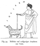
- Melitan: A melitan was a breed of lapdog popular with Romans and Greeks in ancient times. They were small companion dogs, typically pampered things who existed solely to amuse their owners, typically noblewomen. "The Melitan was a small, fluffy, spitz-type dog, commonly white in colour... with a very appealing, pointed, fox-like muzzle." In appearance, they sound nothing like Dogmatix. But the Melitan hypothesis is very strong for another reason: these small dogs actually existed as pets in 50BC. There's no record of them amongst Gauls, however. We'd have to imagine that rowdy, warring Obelix came into possession of a small Roman lapdog during a raid.

- A Gallic war dog, a.k.a. Irish Wolfhound: What we call an Irish wolfhound is a very ancient breed of dog which Celts were known to use as guard dogs and in combat. Caesar is supposed to have mentioned them in his Commentaries on the Gallic War, though I couldn't find the reference. This is the only breed of dog which we might realistically find in a Gaulish village in 50BC, which makes it a good hypothesis for Dogmatix. The obvious flaw: wolfhounds are huge. Maybe Dogmatix could be a wolfhound, but he'd have to be an anemic, albino, malformed runt of a wolfhound. He is known to accompany Obelix on raids and bite Romans.

- Schnauzer: The last hypothesis: Dogmatix could be a schnauzer. This is unlikely for so many reasons: (1) schnauzers didn't exist in 50BC; (2) they aren't native to Gaul/France; (3) they look nothing like Dogmatix except, except, except that schnauzers have whiskers that perhaps vaguely resemble Dogmatix's unusual moustache.
Which breed does Dogmatix belong to...?
Our goal is to determine which of these four breeds Dogmatix belongs to. First, we need some data, then we need a method for decision making.
The data: despite Romans being fastidious record keepers, no survey of dog measurements exists from ancient times. I've generated twenty height and weight measurements for each breed. The data is fictional, but it's generated using the best estimates of typical dimensions I could find on the web (eg. wikipedia).
Note: as is often the case with Python (or, at least, with my amateurish Python), the code required to create the charts is 3x the length of the code that does the actual computations. In the code below, I've marked where the visualisation sections begin with #### CHARTS #### so that the disinterested reader can easily skip them (the disinterested reader should feel free to skip all the code, if desired...)
# prepare Python
%pylab inline
from scipy import stats
import numpy as np
import pandas as pd

from matplotlib._png import read_png
from matplotlib.offsetbox import OffsetImage, AnnotationBbox

# create dictionary of breeds, with ((mean heigh, SD height),(mean weight, SD weight))
breeddict = {}
breeddict['Terrier'] = ((38.5,1.25),(7.95,0.575))
breeddict['Melitan'] = ((29.2,0.65),(5.05,0.225))
breeddict['Schnauzer'] = ((48.5,0.75),(6.6,0.8))
breeddict['Wolfhound'] = ((54.6,1.1),(11.6,1.75))
listBreeds = breeddict.keys()

# create a colour palette
listColours = ['red','blue','green','orange']

# function to create random height & weight observations for a dog breed
# Because there is going to be a correlation between height & weight, we let that reflect in covariance
np.random.seed(123)
def dogobs(breed):
    ((muheight,sdheight),(muweight,sdweight)) = breeddict[breed]
    cov1=np.random.randint(1,3)
    cov2=np.random.randint(1,20)
    observations = np.random.multivariate_normal([muheight, muweight], [[sdheight**2, cov1],[cov2, sdweight**2]], 30)
    obsdf = pd.DataFrame(data=observations,columns=['height','weight'])
    obsdf['breed'] = breed
    return obsdf

# create a dataframe with 30 observations for each breed
dogsdf = pd.DataFrame(columns=['height','weight','breed'])
for breed in listBreeds:
    obsdf = dogobs(breed)
    dogsdf = dogsdf.append(obsdf)

#### CHARTS ####
fig = plt.figure(figsize(16,6), dpi=1600) # specifies the parameters of our graphs
plt.subplots_adjust(hspace=.5)            # extra space between plots
gridsize = (2,2)

# scatterplot of dogs by height and weight
ax0 = plt.subplot2grid(gridsize,(0,0),rowspan=2)
for breed, colour in zip(listBreeds,listColours):
    dogset = dogsdf[dogsdf['breed']==breed]
    ax0.scatter(dogset['height'], dogset['weight'], c=colour, label=breed, s=35, alpha=.6)
ax0.set_xlabel('height')
ax0.set_ylabel('weight')
ax0.set_title('Observations of dog breeds')
ax0.legend(loc=2)

# plot univariate distribution of height
grouped = dogsdf.groupby('breed');
ax1 = plt.subplot2grid(gridsize,(0,1))
for breed, colour in zip(listBreeds,listColours):
    dogset = dogsdf[dogsdf['breed']==breed]
    dogset['height'].plot(kind='kde', ax=ax1, c=colour);
ax1.set_xlabel('height')
ax1.set_title('height probability densities')

# plot univariate distribution of weight
ax2 = plt.subplot2grid(gridsize,(1,1))
for breed, colour in zip(listBreeds,listColours):
    dogset = dogsdf[dogsdf['breed']==breed]
    dogset['weight'].plot(kind='kde', ax=ax2, c=colour);
ax2.set_xlabel('weight')
ax2.set_title('weight probability densities')

# Add dogmatix to charts
heightDogmatix = 37
weightDogmatix = 6

## add to scatterplot
ax0.scatter(heightDogmatix,weightDogmatix,c='white',s=150)
dogmatixfile = 'Dogmatix.png'
imdogmatix = plt.imread(dogmatixfile)
imagebox = OffsetImage(imdogmatix, zoom=0.25)
ab = AnnotationBbox(imagebox, (heightDogmatix,weightDogmatix), xybox=(25,10),
                    arrowprops=dict(arrowstyle="->", connectionstyle="angle,angleA=90,angleB=0,rad=3"));
ax0.add_artist(ab);

The dimensions of Dogmatix
I should quickly explain how I came up with Dogmatix's height and weight:
- Height: According to the internet, Julius Caesar was 5'7. If you take a ruler and measure the height of JC in an Asterix comic, and the height of Dogmatix, then you can calculate that Dogmatix must be around 37cm tall.
- Weight: I asked a veterinarian friend of mine to guess. She guessed 6kg.
Much like our gaulish village, Dogmatix falls into a disputed region at the intersection of the Schnauzer, Terrier and Melitan breeds.
Bayesian classification
We are classifying dogs into breeds according to height and weight. Our task is to build a model which, given a height & weight, will return the most likely dog breed. One way to do that is to calculate Pr(breed|height,weight): that is, calculate the probability of a dog being a schnauzer or a terrier or a wolfhound given a certain height and weight.
Bayes' rule is one method to do so. This is Bayes' rule:
$Pr(class|data)=\frac{\Pr(data|class)\Pr(class)}{\Pr(data)}$
This is Bayes' rule expressed in terms of our dog breed classification problem:
$Pr(breed|height, weight)=\frac{\Pr(height, weight|breed)\Pr(breed)}{\Pr(height, weight)}$
What does it mean? Bayes' rule provides an easy way to calculate Pr(class|data), the term on the left-hand side. In our case, we want to know Pr(breed|height, weight). Once we have that, we can clasify Dogmatix into a breed using his height (37cm) and weight (6kg). For many problems, calculating Pr(class|data) can be difficult or computationally intensive, which is why traditional 'Frequentist' statistical methods usually aim instead for Pr(data|class).
How does Bayes' rule work? The best explanation is an example. We'll work through each of the components on the right-hand side of the formula below, and then we'll use the formula to calculate the Pr(class|data).

Where does it come from? Bayes' rule first appeared in a paper by the Reverend Thomas Bayes, a Presbyterian minister whose writings to date had tended towards the theological (eg. Divine Benevolence, or an Attempt to Prove That the Principal End of the Divine Providence and Government is the Happiness of His Creatures (1731)). His paper talked a lot about throwing billiard balls onto tables and calculating how far from the edge they might land. It was never published in his lifetime - it was discovered amongst his possessions by a friend after he died and published in 1764 in Philosophical Transactions of the Royal Society of London. It was then subsequently forgotten. In 1774 the rule was discovered all over again by Napoleonic-era genius Pierre-Simon Laplace, who went on to use it in many problems. (Since Laplace also discovered the rule, and did the most to popularise it, you might think it is a shame that it isn't named after him. He can take consolation in knowing that Wikipedia has a dedicated list of things named after Laplace).
Step 1: Specify Pr(breed), the 'prior'
In Bayes' rule, the term Pr(class) is called the 'prior'. It's the prior probability of each class - in this case, dog breed. What are the chances of seeing a westie or a schnauzer in a Gaulish village around 50BC? Very slim, I would say. What are the chances of seeing a melitan or a wolfhound? Much better.
This is our easiest and yet most anguishing task. Plainly, without some sort of census of dog breeds from 50BC, this is going to involve some guesswork.
pSchnauzer = 0.1     # very unlikely
pWolfhound = 0.5     # Potential - actually kept by Gauls, though bares little resemblance to Dogmatix
pTerrier = 0.1       # very unlikely
pMelitan = 0.3       # Potential - captured by Obelix from Romans

#### CHARTS ####
fig = plt.figure(figsize(6,4), dpi=1600)
plt.axes(frameon=False)
ind = np.arange(4)
width = 0.75
for (ind, prob, colour) in zip(ind,[pSchnauzer, pWolfhound, pTerrier, pMelitan],listColours):
    plt.bar(ind, prob, width, color=colour, alpha=0.5, linewidth=0);
    plt.text(ind+width/2, prob+0.01, "{0:.0f}%".format(prob * 100), va='bottom', ha='center') ;

plt.ylim(0,0.6)
plt.xlim(-0.25,None)
plt.xticks([i+width/2 for i in np.arange(4)],listBreeds);

# formatting
plt.tick_params(axis='x', which='both', bottom='off', top='off', labelbottom='on')
plt.tick_params(axis='y', which='both', left='off', right='off', labelleft='off')
plt.title("Prior probabilities for each breed")

Note that we could have specified more complicated priors - perhaps ones that vared across height & weight: I don't know enough about dogs to do this, so let's stick with flat probabilities for each breed.
Step 2: Specify Pr(height, weight | class), the 'likelihood'
The likelihood is the joint weight & height probability distribution within each dog breed. We derive this from our data.
There are various assumptions that we can make to simplify this task. Naive Bayesian approaches assume all variables are independant. Gaussian approaches assume variables are normally distributed. I'd like to avoid any assumptions and instead use kernel density estimation to estimate a multivariate height & weight distribution within each class. Departing from parametric distributions creates new difficulties, which we'll skirt around by discrete-ising the problem space into a 100x100 grid.
from sklearn.neighbors.kde import KernelDensity
from mpl_toolkits.mplot3d import Axes3D

# use KDE to get joint distribution across height, weight within each class
KDESchnauzer = KernelDensity(kernel='gaussian', bandwidth=2).fit(dogsdf[dogsdf['breed']=='Schnauzer'][['height','weight']])
KDEWolfhound = KernelDensity(kernel='gaussian', bandwidth=2).fit(dogsdf[dogsdf['breed']=='Wolfhound'][['height','weight']])
KDETerrier = KernelDensity(kernel='gaussian', bandwidth=2).fit(dogsdf[dogsdf['breed']=='Terrier'][['height','weight']])
KDEMelitan = KernelDensity(kernel='gaussian', bandwidth=2).fit(dogsdf[dogsdf['breed']=='Melitan'][['height','weight']])

## calculate p(height,weight | breed) for each point in our decision space
# define decision space
rangeHeight = np.linspace(20,65,100)
rangeWeight = np.linspace(2,16,100)
X, Y = np.meshgrid(rangeHeight, rangeWeight)

# calculate p(class | data) joint distributions across decision region (X,Y)
pDataGivenSchnauzer = np.exp(KDESchnauzer.score_samples(np.c_[X.ravel(), Y.ravel()])).reshape(X.shape)
pDataGivenWolfhound = np.exp(KDEWolfhound.score_samples(np.c_[X.ravel(), Y.ravel()])).reshape(X.shape)
pDataGivenTerrier = np.exp(KDETerrier.score_samples(np.c_[X.ravel(), Y.ravel()])).reshape(X.shape)
pDataGivenMelitan = np.exp(KDEMelitan.score_samples(np.c_[X.ravel(), Y.ravel()])).reshape(X.shape)

#### CHARTS ####
fig = plt.figure(figsize(10,8), dpi=1600) # specifies the parameters of our graphs
plt.subplots_adjust(hspace=.5)            # extra space between plots

ax1 = plt.subplot2grid((2,2),(0,0), projection='3d')
ax1.plot_surface(X, Y, pDataGivenSchnauzer, rstride=5, cstride=5, cmap=cm.Reds)
ax1.contourf(X, Y, pDataGivenSchnauzer, zdir='x', offset=65, cmap=cm.Reds)
ax1.contourf(X, Y, pDataGivenSchnauzer, zdir='y', offset=16, cmap=cm.Reds)
ax1.view_init(azim=240, elev=30)
ax1.set_zlim(0,0.02)
plt.title("Joint Likelihood\n p(height,weight | breed = schnauzer)")

ax2 = plt.subplot2grid((2,2),(0,1), projection='3d')
ax2.plot_surface(X, Y, pDataGivenWolfhound, rstride=5, cstride=5, cmap=cm.Blues)
ax2.contourf(X, Y, pDataGivenWolfhound, zdir='x', offset=65, cmap=cm.Blues)
ax2.contourf(X, Y, pDataGivenWolfhound, zdir='y', offset=16, cmap=cm.Blues)
ax2.view_init(azim=240, elev=30)
ax2.set_zlim(0,0.02)
plt.title("Joint Likelihood\n p(height,weight | breed = wolfhound)")

ax3 = plt.subplot2grid((2,2),(1,0), projection='3d')
ax3.plot_surface(X, Y, pDataGivenTerrier, rstride=5, cstride=5, cmap=cm.Greens)
ax3.contourf(X, Y, pDataGivenTerrier, zdir='x', offset=65, cmap=cm.Greens)
ax3.contourf(X, Y, pDataGivenTerrier, zdir='y', offset=16, cmap=cm.Greens)
ax3.view_init(azim=240, elev=30)
ax3.set_zlim(0,0.02)
plt.title("Joint Likelihood\n p(height,weight | breed = terrier)")

ax4 = plt.subplot2grid((2,2),(1,1), projection='3d')
ax4.plot_surface(X, Y, pDataGivenMelitan, rstride=5, cstride=5, cmap=cm.Oranges)
ax4.contourf(X, Y, pDataGivenMelitan, zdir='x', offset=65, cmap=cm.Oranges)
ax4.contourf(X, Y, pDataGivenMelitan, zdir='y', offset=16, cmap=cm.Oranges)
ax4.view_init(azim=240, elev=30)
ax4.set_zlim(0,0.02)
plt.title("Joint Likelihood\n p(height,weight | breed = melitan)")

The four 3D charts show the joint height-weight probability distributions within each of the dog breeds.
If we were to use the likelihoods to make decisions, we could construct decsion boundaries by allocating height/weight points to the class with the highest likelihood. You will see that this would place Dogmatix in the westie breed:
# Calculate which class has higher likelihood at each point
def comparethem(a,b,c,d):
    return [a,b,c,d].index(max(a,b,c,d))

Zclass = []
Zclass = array([comparethem(a,b,c,d) for a,b,c,d in zip(pDataGivenSchnauzer.ravel(),pDataGivenWolfhound.ravel(),
                                                        pDataGivenTerrier.ravel(),pDataGivenMelitan.ravel())])
Zclass = Zclass.reshape(X.shape)

# create matrix which contains the max likelihood at each point
Z = array([max(i,j,k,l) for i,j,k,l in zip(pDataGivenSchnauzer.ravel(),pDataGivenWolfhound.ravel(),
                                           pDataGivenTerrier.ravel(),pDataGivenMelitan.ravel())])
Z = Z.reshape(X.shape)

fig = plt.figure(figsize(18,6), dpi=1600) # specifies the parameters of our graphs
plt.subplots_adjust(hspace=.5)            # extra space between plots

# plot 3d chart of max posterior probability, coloured by source breed
Zclass2 = array([listColours[i] for i in Zclass.ravel()] )
Zclass2 = Zclass2.reshape(X.shape)
ax1 = plt.subplot2grid((1,2),(0,0), projection='3d')
ax1.view_init(azim=230, elev=30)
ax1.plot_surface(X, Y, Z, rstride=4, cstride=4, facecolors=Zclass2, shade=True, alpha=0.3)
ax1.set_title("Joint likelihoods for all breeds\n p(height,weight|breed)")

# plot overhead map of decision regions
from matplotlib import colors as c
cMap = c.ListedColormap(listColours)  # custom colour map necessary for colormesh
ax2 = plt.subplot2grid((1,2),(0,1))
ax2.pcolormesh(X, Y, Zclass, cmap=cMap, alpha=0.1)
for breed, colour in zip(listBreeds,listColours):
    dogset = dogsdf[dogsdf['breed']==breed]
    ax2.scatter(dogset['height'], dogset['weight'], c=colour, label=breed, s=35, alpha=.6)
ax2.set_title("Maximum likelihood decision regions for each breed")
ax2.set_xlim(min(rangeHeight),max(rangeHeight))
ax2.set_ylim(min(rangeWeight),max(rangeWeight))
ax2.legend(loc=2)

# Add dogmatix
ax2.scatter(heightDogmatix,weightDogmatix,c='white',s=150)
dogmatixfile = 'Dogmatix.png'
imdogmatix = plt.imread(dogmatixfile)
imagebox = OffsetImage(imdogmatix, zoom=0.25)
ab = AnnotationBbox(imagebox, (heightDogmatix,weightDogmatix), xybox=(25,10),
                    arrowprops=dict(arrowstyle="->", connectionstyle="angle,angleA=90,angleB=0,rad=3"));
ax2.add_artist(ab);

Step 3: Calculate Pr(class | data), the 'posterior'
Now the magic of Bayes. To calculate Pr(class | data) we use Bayes' rule:
$Pr(class|data)=\frac{\Pr(data|class)\Pr(class)}{\Pr(data)}$
We're multiplying together the prior and the likelihood probability distributions which we've just defined above. We divide by the constant term Pr(data), which is the sum of Pr(data|class)*Pr(class) across all clases. The Pr(data) term is a constant, it serves to normalise the posterior probability distribution so it sums to 1. For this reason it isn't very interesting. It is often omitted in machine learning implementations of Bayes since it is a constant and thus has no bearing on the relative ranking of classes in the posterior.
# calculate 'evidence' term = constant to normalise everything to sum to 1
p_data= sum(pDataGivenTerrier * pTerrier) + sum(pDataGivenMelitan * pMelitan) + sum(pDataGivenSchnauzer * pSchnauzer) + sum(pDataGivenWolfhound * pWolfhound)

pTerrierGivenData = pDataGivenTerrier * pTerrier / p_data
pMelitanGivenData = pDataGivenMelitan * pMelitan / p_data
pSchnauzerGivenData = pDataGivenSchnauzer * pSchnauzer / p_data
pWolfhoundGivenData = pDataGivenWolfhound * pWolfhound / p_data

#### CHARTS ####
# create matrix which contains the max posterior probability at each point
Z = array([max(i,j,k,l) for i,j,k,l in zip(pSchnauzerGivenData.ravel(),pWolfhoundGivenData.ravel(),
                                        pTerrierGivenData.ravel(),pMelitanGivenData.ravel())])
Z = Z.reshape(X.shape)

# create matrix that includes which breed had max posterior probability at each point
Zclass = []
Zclass = array([comparethem(a,b,c,d) for a,b,c,d in zip(pSchnauzerGivenData.ravel(), pWolfhoundGivenData.ravel(),
                                             pTerrierGivenData.ravel(), pMelitanGivenData.ravel())])
Zclass = Zclass.reshape(X.shape)

fig = plt.figure(figsize(18,6), dpi=1600) # specifies the parameters of our graphs
plt.subplots_adjust(hspace=.5)            # extra space between plots

# plot 3d chart of max posterior probability, coloured by source breed
Zclass2 = array([listColours[i] for i in Zclass.ravel()] )
Zclass2 = Zclass2.reshape(X.shape)
ax1 = plt.subplot2grid((1,2),(0,0), projection='3d')
ax1.view_init(azim=230, elev=30)
ax1.plot_surface(X, Y, Z, rstride=4, cstride=4, facecolors=Zclass2, shade=True, alpha=0.3)
ax1.set_title("Maximum a posteriori probability by breed\n p(breed | height,weight)")

# plot overhead map of decision regions
from matplotlib import colors as c
cMap = c.ListedColormap(listColours)  # custom colour map necessary for colormesh
ax2 = plt.subplot2grid((1,2),(0,1))
ax2.pcolormesh(X, Y, Zclass, cmap=cMap, alpha=0.1)
for breed, colour in zip(listBreeds,listColours):
    dogset = dogsdf[dogsdf['breed']==breed]
    ax2.scatter(dogset['height'], dogset['weight'], c=colour, label=breed, s=35, alpha=.6)
ax2.set_title("Maximum a posterior decision regions for each breed")
ax2.set_xlim(min(rangeHeight),max(rangeHeight))
ax2.set_ylim(min(rangeWeight),max(rangeWeight))
ax2.legend(loc=2)

# Add dogmatix
ax2.scatter(heightDogmatix,weightDogmatix,c='white',s=150)
dogmatixfile = 'Dogmatix.png'
imdogmatix = plt.imread(dogmatixfile)
imagebox = OffsetImage(imdogmatix, zoom=0.25)
ab = AnnotationBbox(imagebox, (heightDogmatix,weightDogmatix), xybox=(25,10),
                    arrowprops=dict(arrowstyle="->", connectionstyle="angle,angleA=90,angleB=0,rad=3"));
ax2.add_artist(ab);

Look at the left-hand 3D posterior probability distribution. I hope you can visualise how this is the result of multiplying the four Pr(breed) priors in Step 1 with the four Pr(height, weight|breed) likelihood distributions in Step 2.
So Dogmatix is a...?

Now we have a posterior distribution for Pr(breed|height, weight), so we can classify Dogmatix into the class which has the highest probability at his height & weight. The decision regions can be seen in the right-hand chart. The technical term is the maximum a posteriori.

If we had classified Dogmatix using the likelihood distribution from Step 2 then we would probably have concluded that he was a terrier. However, the posterior distribution tells a different story. Accounting for the fact that it would be very unlikely to find a terrier in ancient Gaul, our maximum a posteriori classification for Dogmatix is a melitan, the breed of small lapdogs popular with ancient Romans.
Bayesian reasoning is an interplay between the prior and the likelihood distributions. I hope it's clear how the prior has influenced the posterior. Although the likelihood distributions of the three classes were of similar size and shape, the 30% prior for the melitan breed has expanded the decision boundary for that breed at the expense of the terrier.
Conclusion: On the influence of the prior
There continues to be raging debate over Bayesian vs Frequentist statistics and their respective philosophies of probability. The (arguably) subjective nature of the Bayesian prior is a major point of contention. One can imagine how the classification of Dogmatix could have turned out differently given a different set of priors. Intuitively, we want our statistics to be objective, particularly if they are used for science. I don't think a Bayesian would deny that there is subjectivity to their method, but I think they would counter that there is just as much subjectivity in Frequentist statistics - it's just better concealed.
From a strictly pragmatic point of view, the benefit of the Bayesian approach is that it can incorporate contextual knowledge via the prior. If you have a problem where your class priors are all the same then you might find that the Bayesian approach adds little but mathematical overhead. But if you have a problem where class priors are an important feature - like in this case - then the Bayesian approach has unique advantages.
For the reader interested in where Bayesian methods have proved very effective, Peter Norvig's demonstration of how Google's spelling auto-suggest function works is excellent. Note how the prior plays a crucial role.

Postscript: just for fun, let's see how a few other popular classification systems would classify Dogmatix:
# encode breeds to facilitate easier processing
breedcode = {'Schnauzer' : 0, 'Wolfhound' :  1, 'Terrier': 2, 'Melitan' : 3}
dogsdf['breedcode'] = dogsdf['breed'].apply(breedcode.get)

fig = plt.figure(figsize(15,15), dpi=1600) # specifies the parameters of our graphs
plt.subplots_adjust(hspace=.3)             # extra space between plots
mycmap = c.ListedColormap(listColours)     # custom colour map necessary for colormesh

nrows = 3
ncols = 3
gridsize = (nrows,ncols)
plotspots = [(i,j) for i in range(nrows) for j in range(ncols)]

def plotcases(ax):
    for breed, colour in zip(listBreeds,listColours):
        dogset = dogsdf[dogsdf['breed']==breed]
        ax.scatter(dogset['height'], dogset['weight'], c=colour, label=breed, s=35, alpha=.6)
        ax.scatter(heightDogmatix,weightDogmatix,c='white',s=150, alpha=0.6)
        plt.xlim(20,65)
        plt.ylim(2,16)

# base problem
ax0 = plt.subplot2grid(gridsize,plotspots[0])
plotcases(ax0)
ax0.title.set_text("The problem...")
dogmatixfile = 'Dogmatix.png'
imdogmatix = plt.imread(dogmatixfile)
imagebox = OffsetImage(imdogmatix, zoom=0.2)
ab = AnnotationBbox(imagebox, (heightDogmatix,weightDogmatix), xybox=(26.5,12.5),
                    arrowprops=dict(arrowstyle="->", connectionstyle="angle,angleA=90,angleB=0,rad=3"));
ax0.add_artist(ab);

# kNN, k=5
from sklearn import neighbors
knn5 = neighbors.KNeighborsClassifier(n_neighbors=3)
knn5.fit(dogsdf[['height','weight']], dogsdf['breedcode'])
Z = knn5.predict(np.c_[X.ravel(), Y.ravel()])
Z = Z.reshape(X.shape)
ax1 = plt.subplot2grid(gridsize,plotspots[1])
ax1.title.set_text("kNN, k=3")
ax1.pcolormesh(X, Y, Z, cmap=mycmap, alpha=0.1)
plotcases(ax1)

# kNN, k=10
knn10 = neighbors.KNeighborsClassifier(n_neighbors=10)
knn10.fit(dogsdf[['height','weight']], dogsdf['breedcode'])
Z = knn10.predict(np.c_[X.ravel(), Y.ravel()])
Z = Z.reshape(X.shape)
ax2 = plt.subplot2grid(gridsize,plotspots[2])
ax2.title.set_text("kNN, k=10")
ax2.pcolormesh(X, Y, Z, cmap=mycmap, alpha=0.1)
plotcases(ax2)

# SVCs
from sklearn import svm
svc1 = svm.SVC(kernel='linear')
svc1.fit(dogsdf[['height','weight']], dogsdf['breedcode'])
Z = svc1.predict(np.c_[X.ravel(), Y.ravel()])
Z = Z.reshape(X.shape)
ax3 = plt.subplot2grid(gridsize,plotspots[3])
ax3.title.set_text("SVM, linear")
ax3.pcolormesh(X, Y, Z, cmap=mycmap, alpha=0.1)
plotcases(ax3)

svc2 = svm.SVC(kernel='poly',degree=4)
svc2.fit(dogsdf[['height','weight']], dogsdf['breedcode'])
Z = svc2.predict(np.c_[X.ravel(), Y.ravel()])
Z = Z.reshape(X.shape)
ax4 = plt.subplot2grid(gridsize,plotspots[4])
ax4.title.set_text("SVM, 4th order polynomial")
ax4.pcolormesh(X, Y, Z, cmap=mycmap, alpha=0.1)
plotcases(ax4)

svc3 = svm.SVC(kernel='rbf')
svc3.fit(dogsdf[['height','weight']], dogsdf['breedcode'])
Z = svc3.predict(np.c_[X.ravel(), Y.ravel()])
Z = Z.reshape(X.shape)
ax5 = plt.subplot2grid(gridsize,plotspots[5])
ax5.title.set_text("SVM, radial basis function")
ax5.pcolormesh(X, Y, Z, cmap=mycmap, alpha=0.1)
plotcases(ax5)

# Decision tree
from sklearn import tree
dtree = tree.DecisionTreeClassifier()
dtree = dtree.fit(dogsdf[['height','weight']], dogsdf['breedcode'])
Z = dtree.predict(np.c_[X.ravel(), Y.ravel()])
Z = Z.reshape(X.shape)
ax6 = plt.subplot2grid(gridsize,plotspots[6])
ax6.title.set_text("Decision tree")
ax6.pcolormesh(X, Y, Z, cmap=mycmap, alpha=0.1)
plotcases(ax6)

# Gaussian Naive Bayes with learned priors
from sklearn.naive_bayes import GaussianNB
gnb = GaussianNB()
gnb.fit(dogsdf[['height','weight']], dogsdf['breedcode'])
Z = gnb.predict(np.c_[X.ravel(), Y.ravel()])
Z = Z.reshape(X.shape)
ax7 = plt.subplot2grid(gridsize,plotspots[7])
ax7.title.set_text("Gaussian Naive Bayes")
ax7.pcolormesh(X, Y, Z, cmap=mycmap, alpha=0.1)
plotcases(ax7)
