
Today's post is going to be a bit more abstract and a bit less applied than usual, because today I want to take Python's Sympy symbolic algebra library for a spin. As a narrative subject, we'll be looking at the medieval English Longbow. We'll start with some physics by modelling the deterministic trajectory of the arrow. Then we'll add some statistical noise to make it a bit more realistic. Lastly, we'll do some simple Bayesian inference on the range of the longbow. And we'll do as much of it as we can via symbolic algebra.
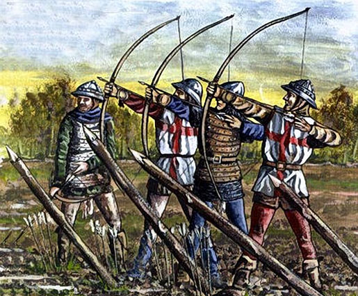
These are English longbowmen. The English (or Welsh) Longbow is around 1.8-2m tall, can fire 10-12 arrows per minute in the hands of a skilled archer, and its steel-tipped arrows can penetrate the armour of a medieval knight. The "draw-weight" of a longbow is considerable, and skeletons of longbow archers often have enlarged left arms. Over a lifetime, the archer's body was actually deformed by their tool of trade. So, how far could it shoot an arrow? Let's figure that out with physics. According to Longbow Speed Testing (!), the velocity of an arrow leaving the bow is 172-177 feet per second. Say 53m/s in metric.
The trajectory of a projectile can be computed using classical mechanics:
$y = x \tan{\left (\alpha \right )} - \frac{g x^{2}}{2 v^{2} \cos^{2}{\left (\alpha \right )}}$
Where:
- $y$ is the height of the arrow
- $x$ is the horizontal distance that the arrow has travelled
- $\alpha$ is the angle at which the arrow is fired
- $v$ is the velocity of the arrow as it leaves the bow
- $g$ is the acceleration due to gravity (~$9.8 m/s^2$ on the surface of the earth)
- (We're ignoring wind resistance)
Let's start by loading this into Sympy:
## Prepare Python & IPython Notebook
%pylab inline
from sympy import init_printing; init_printing()

import numpy as np
from sympy import *
from sympy.stats import *

## Define our symbols
alpha = Symbol('alpha')  # angle
v = Symbol('v')          # velocity
g = Symbol('g')          # gravity
x = Symbol('x')          # distance

## Projectile equation
y = x * tan(alpha) - (g * x**2) / ( 2 * (v * cos(alpha))**2 )
y
$- \frac{g x^{2}}{2 v^{2} \cos^{2}{\left (\alpha \right )}} + x \tan{\left (\alpha \right )}$
Sympy outputs our equation already nicely formatted using Mathjax. Lovely! So, now we have the equation for projectile motion in Sympy. (Sympy has a strange habit of putting negative terms first, but it's still the same equation).
The simplest thing we can do is substitute in values. Let's start by setting:
- gravity ($g$) = 9.8
- angle ($\alpha$) = 45 degrees ($\frac{\pi}{4}$)
- velocity ($v$) = 53 m/s
y.subs({g:9.8, alpha:pi/4, v:53})
$- 0.00348878604485582 x^{2} + x$
Giving us an equation for the height of the arrow at any distance. Which we should plot:
plot(y.subs({g:9.8, alpha:pi/4, v:53}), (x, 0, 350))

Impact would be, of course, when the height ($y$) returns to 0. Let's have Sympy work out when that is:
solve(y.subs({g:9.8, alpha:pi/4, v:53}))
[0.0, 286.632653061225]
Impact at 287m. Sympy can differentiate for us, too. So we could work out the distance at which the arrow reaches peak height (which is vertex of the parabola) by differentiating, setting to zero, and solving for $x$:
dydx = diff(y, x)
dydx
$- \frac{g x}{v^{2} \cos^{2}{\left (\alpha \right )}} + \tan{\left (\alpha \right )}$
max_height = solve(dydx, x)
max_height
$\begin{bmatrix}\frac{v^{2}}{2 g} \sin{\left (2 \alpha \right )}\end{bmatrix}$
solve(diff(y.subs({g:9.8, alpha:pi/4, v:53}), x))
[143.316326530612]
So we can calculate the range and trajectory of an idealised medieval longbow without too much trouble. But it's not realistic to expect that every arrow would follow the same trajectory and land exactly 287m away. One would expect that the impact range would vary given variations in the archer's angle of elevation and arrow velocity. In Sympy, we could make each of these variables random variables, thereby introducing some statistical noise.
Let's re-specify our trajectory formula, but with these changes:
- $v \sim \mathcal{N} (53,5^2)$ : Arrow velocity as a normally distributed variable with mean 53 and standard deviation of 5
- $\alpha \sim \mathcal{N} (\frac{\pi}{4}, \frac{\pi}{16}^2)$ : Angle of departure as normally distributed with mean 45 degrees and standard deviation of 11.25 degrees
- $g$ = 9.8: fix gravity to be 9.8
And now each arrow will follow slightly different trajectories:
# Specify variables
v = Normal('v', 53, 5)
alpha = Normal('alpha', pi/4, pi/16)
g = 9.8

# Define function for arrow height given variables
y = x * tan(alpha) - (g * x**2) / ( 2 * (v * cos(alpha))**2 )

# plot 10 arrows with randomly selected angles & velocities
fig = plt.figure(figsize(6,2))
plot(y.subs({alpha:sample(alpha), v:sample(v)}),
     y.subs({alpha:sample(alpha), v:sample(v)}),
     y.subs({alpha:sample(alpha), v:sample(v)}),
     y.subs({alpha:sample(alpha), v:sample(v)}),
     y.subs({alpha:sample(alpha), v:sample(v)}),
     y.subs({alpha:sample(alpha), v:sample(v)}),
     y.subs({alpha:sample(alpha), v:sample(v)}),
     y.subs({alpha:sample(alpha), v:sample(v)}),
     y.subs({alpha:sample(alpha), v:sample(v)}),
     y.subs({alpha:sample(alpha), v:sample(v)}),
     (x, 0, 400), ylim=(0,200))

We can work out a function for the range by solving for those points where the height (y) is 0:
xland = solve(y,x)[1]
xland
$0.102040816326531 \sin{\left (2.0 \alpha \right )} v^{2}$
Which looks like a simple formula, but don't forget that $\alpha$ and $v$ are both random variables. And that makes the range a random variable, too, so let's call it $\theta$. Which means that we can ask statistical questions of it, What is the expected (mean) range?
E(xland).evalf()
267.723772725618
In symbolic/analytic terms, what Sympy is doing is solving this hideous looking double integral:
E(xland, evaluate=False)
$\int_{-\infty}^{\infty} \frac{\sqrt{2}}{10 \sqrt{\pi}} e^{- \frac{1}{50} \left(v - 53\right)^{2}} \int_{-\infty}^{\infty} \frac{0.816326530612245 \sqrt{2}}{\pi^{\frac{3}{2}}} v^{2} e^{- \frac{128}{\pi^{2}} \left(\alpha - \frac{\pi}{4}\right)^{2}} \sin{\left (2.0 \alpha \right )}\, d\alpha\, dv$
... and that's pretty cool. Perhaps more interestingly we can ask, What is the probability that an arrow flies more than 300m?:
P(xland>300)
$\int_{0}^{\infty}\int_{-\infty}^{\infty} \frac{\sqrt{2}}{10 \sqrt{\pi}} e^{- \frac{1}{50} \left(v - 53\right)^{2}} \int_{-\infty}^{\infty} \frac{8 \sqrt{2}}{\pi^{\frac{3}{2}}} e^{- \frac{128}{\pi^{2}} \left(\alpha - \frac{\pi}{4}\right)^{2}} \delta\left(- z + 0.102040816326531 v^{2} \sin{\left (2.0 \alpha \right )} - 300\right)\, d\alpha\, dv\, dz$
Here Sympy has been unable to compute the result and has instead returned an unresolved integral. The infinite integration range wasn't the problem, either, as I tried giving it concrete ranges to integrate over. It's a little hard to know whether Sympy deserves any criticism here. There's many integrals that are intractable, which loosely means that they cannot be expressed in terms of simple functions with known integration procedures. My calculus is not very strong and simply from looking at this I can't say for certain whether it is intractable or not. Happily, Sympy has built-in Monte Carlo estimation. It provides a quick means to estimate troublesome integrals like this:
P(xland>300, numsamples=10000)
0.2872
Seeing as I was unable to do the necessary integration required to evaluate a probability, I was unable to resolve both $v$ and $\alpha$ random variables into a PDF for range ($X$). We already have the expectation, and we can ask Sympy to calculate the standard deviation, too, which together give us a good idea.
sqrt(variance(xland, numsamples=10000))
58.3808670570045
If we want to get a picture of the final distribution from Sympy, we could do a whole lot of Monte Carlo simulations across the range of $X$ that is interesting:
rangex = np.linspace(0, 500, 40)
v1 = [P(xland<i, numsamples=5000) for i in rangex]
v2 = [0] + [x - v1[i - 1] for i, x in enumerate(v1)][1:]
plt.plot(rangex, v2)
plt.ylim((0,0.1));

Using Bayesian inference to learn how far the longbow can fire arrows
The longbow was terrifically effective for the English during the first half of the hundred years' war. French armies initially didn't know how to combat them. At the Battle of Crécy in 1346, the English army was roughly one-third the size of the French. The French fielded 10,000 knights to the English's 2,500. However, the English brought 5,500 longbowmen and, as a result, the French were swiftly routed, losing 2,000 of their armoured knights.

So, let's turn our statistical problem around. Say that we're a French knight. We don't know anything about the longbow or the physics of projectiles. We have an idea in our head about how far an arrow can travel. We've never seen a longbow before, but we quickly want to learn their range so we can stay at a safe distance.
We'll take a Bayesian approach, so that each time we observe an arrow we can update our beliefs. We've done this sort of thing a few times before in previous posts, but today we'll try and do it with Sympy's symbolic algebra.
We'll designate:
- $\theta$ = range of the longbow
- $X$ = the distances travelled by observed arrow(s) $x_1,...,x_i$
For continuous random variables, Bayes theorem has it:
$P(\theta | X) = \frac{P(X | \theta) P(\theta)}{P(X)}$ where $P(X) = \int P(X | \theta) P(\theta)\,\mathrm{d}\theta$
$P(\theta | X)$ is what we want: the PDF for the range $\theta$ given a distribution of observed arrows $X$.
Let's start small by observing a single arrow:
The prior: $P(\theta)$
Though we've never seen a longbow before, we've seen many other sorts of bow. Our experience has given us an intuition of the range of bows, and that belief can be expressed as a normal distribution with a mean of $\mu$ and a standard deviation of $\rho$:
## PRIOR
theta = Symbol('theta')
mu = Symbol('mu')
rho = Symbol('rho', positive=True)

prior = Normal('prior',mu,rho)
density(prior)(theta)
$\frac{\sqrt{2}}{2 \sqrt{\pi} \rho} e^{- \frac{\left(- \mu + \theta\right)^{2}}{2 \rho^{2}}}$
To help with intuition, let's see what that would look like if we made it concrete. Say that, in our experience, the range of arrows has a mean of 150m and a standard deviation of 50m. So, $\theta \sim \mathcal{N} (150,50^2)$. We can substitute those values into a prior PDF:
thetarange = np.linspace(0,500,100)
p_theta = [density(prior.subs({mu:150,rho:50}))(theta) for theta in thetarange]

fig = plt.figure(figsize(6,2))
plt.plot(thetarange, p_theta)
plt.title(r'P($\theta$)')

The likelihood: $P(X | \theta)$
A single arrow from a longbow flies over our head, tweaking a realisation that our beliefs not aligned with reality. Let's say the arrow goes $x$ meters. The likelihood function calculates the probability of $x$ given $\theta$, that is, $P(x | \theta)$. To do this, we must make define a PDF for $X$, so we'll say that $X$ is normally distributed with a mean of $\theta$ and a standard deviation of $\sigma$:
## likelihood (for a single x)
x = Symbol('x')
theta = Symbol('theta')
sigma = Symbol('sigma', positive=True)

likelihood = Normal('Xdist',theta, sigma)
density(likelihood)(x)
$\frac{\sqrt{2}}{2 \sqrt{\pi} \sigma} e^{- \frac{\left(- \theta + x\right)^{2}}{2 \sigma^{2}}}$
Let's visualise it as we did above by making it concrete. To keep it simple let's fix the standard deviation $\sigma$ to be 50. Now, let's say that we see the first arrow fly 300m:
thetarange = np.linspace(0,500,100)
p_X_theta = [density(likelihood.subs({theta:i,sigma:50}))(300) for i in thetarange]

fig = plt.figure(figsize(6,2))
plt.plot(thetarange, p_X_theta)
plt.title(r'P($X | \theta$)')

Computing the posterior
Now we have $P(\theta)$ and $P(X | \theta)$ we can go ahead and plug them into Bayes' theorem and update our beliefs for how far arrows can travel:
$P(\theta | X) = \frac{P(X | \theta) P(\theta)}{P(X)}$ where $P(X) = \int P(X | \theta) P(\theta)\,\mathrm{d}\theta$
Let's do the numerator first:
posterior_numerator = density(prior)(theta) * density(likelihood)(x)
posterior_numerator.simplify()
$\frac{1}{2 \pi \rho \sigma} e^{- \frac{\left(\theta - x\right)^{2}}{2 \sigma^{2}} - \frac{\left(\mu - \theta\right)^{2}}{2 \rho^{2}}}$
It can be shown via torturous algebra (see here) that the product of two normal distributions is itself a normal distribution. In our case, it would be parameterised by a mean of $\frac{\sigma^2\mu + \rho^2x}{\rho^2 + \sigma^2}$ and variance $\frac{\rho^2 \sigma^2}{\rho^2 + \sigma^2}$. One can hardly expect Sympy to be able to recognise this fact, but it would be amazing if one day it could.
To calculate the final posterior, we divide that by $\int P(X | \theta) P(\theta)\,\mathrm{d}\theta$:
posterior_denominator = integrate(posterior_numerator.simplify(), (theta,-oo,oo)).simplify()
posterior = posterior_numerator / posterior_denominator
posterior.simplify()
$\frac{\sqrt{2 \rho^{2} + 2 \sigma^{2}}}{2 \sqrt{\pi} \rho \sigma} e^{- \frac{\left(\theta - x\right)^{2}}{2 \sigma^{2}} - \frac{\left(\mu - \theta\right)^{2}}{2 \rho^{2}} + \frac{1}{2 \rho^{2} \sigma^{2} \left(\rho^{2} + \sigma^{2}\right)} \left(\left(\rho^{2} + \sigma^{2}\right) \left(\mu^{2} \sigma^{2} + \rho^{2} x^{2}\right) - \left(\mu \sigma^{2} + \rho^{2} x\right)^{2}\right)}$
An unwieldy expression. We can simplify it by substituing in those concrete values we've used above:
- $\mu$: the mean of the prior is 150m
- $\rho$: the standard deviation of the prior is 50m
- $\sigma$: the standard deviation of the likelihood is 50m
- $x$: the observed arrow flew 300m
Which leaves a function of $\theta$ only:
posterior.subs({mu:150,rho:50,sigma:50,x:300}).simplify()
$\frac{1}{50 \sqrt{\pi}} e^{- \frac{1}{5000} \left(\theta - 300\right)^{2} - \frac{1}{5000} \left(\theta - 150\right)^{2} + \frac{9}{4}}$
We can make sure that it is a proper PDF by checking that it integrates to 1:
integrate(posterior.subs({mu:150,rho:50,sigma:50,x:300}), (theta,-oo,oo)).evalf()
1.0
Tick! Let's find out the maximum a posteriori:
f = diff(posterior.subs({mu:150,rho:50,sigma:50,x:300}).simplify(),theta)
print solve(f, theta)
[225]
And finish by plotting the posterior beside the prior and likelihood:
thetarange = np.linspace(0,500,100)

## plot prior
plt.plot(thetarange, p_theta, label='prior')

## plot likelihood
p_X_theta = [density(likelihood.subs({theta:i,sigma:50}))(300) for i in thetarange]
plt.plot(thetarange, p_X_theta, label='likelihood')

## plot posterior
p_theta_X = [posterior.subs({mu:150, rho:50,sigma:50,x:300,theta:i}).evalf() for i in thetarange]
plt.plot(thetarange, p_theta_X, label='posterior')

plt.legend(framealpha=0.5)
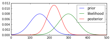
This is just as we'd intuit. Our prior expectation for the range of the longbow, which centered on 150m, has been shifted in the face of evidence. Having seen an arrow fly overhead and land at 300m, our beliefs about the potential range of a bow have moved and now centre at 225m.
One last exercise. Let's see if we can extend this to cover the case where we observe multiple arrows.
Observing multiple arrows

The only thing we need to change is the likelihood $P(X | \theta)$. Instead of observing a single arrow $x$, we now want to observe any number of arrows $x_1,...,x_n$. So we want to calculate $P(x_1,...,x_n | \theta)$, which can be done by:
$P(x_1,...,x_n | \theta) = \prod_{i=1}^n P(x_i | \theta) = \prod_{i=1}^n \frac 1{\sigma\sqrt{2\pi } }e^ { - \frac{(x_i-\theta)^2 }{2 \sigma^2} }$
That's the theory. Problem is that I couldn't figure out how to get Sympy to accept an unspecified number of $x$s in a likelihood formula. So let's make it concrete and just imagine we saw five arrows $x_1,x_2,x_3,x_4,x_5$:
# generate angles & velocities for five random arrows
xs_vars = [(sample(alpha), sample(v)) for i in range(5)]
xs = [int(solve(y.subs({alpha:i, v:j}), x)[1]) for (i, j) in xs_vars]

print "Distance travelled by random arrows: " + str(xs)

fig = plt.figure(figsize(6,2))
plot(y.subs({alpha:xs_vars[0][0], v:xs_vars[0][1]}),
     y.subs({alpha:xs_vars[1][0], v:xs_vars[1][1]}),
     y.subs({alpha:xs_vars[2][0], v:xs_vars[2][1]}),
     y.subs({alpha:xs_vars[3][0], v:xs_vars[3][1]}),
     y.subs({alpha:xs_vars[4][0], v:xs_vars[4][1]}),
     (x, 0, 500), ylim=(0,200))
Distance travelled by random arrows: [255, 269, 304, 212, 288]

Given five observations, the likelihood will be:
## Likelihood for 5 arrows
x_1 = Symbol('x_1')
x_2 = Symbol('x_2')
x_3 = Symbol('x_3')
x_4 = Symbol('x_4')
x_5 = Symbol('x_5')

likelihood_5 = density(likelihood)(x_1)*density(likelihood)(x_2)*density(likelihood)(x_3)*density(likelihood)(x_4)*density(likelihood)(x_5)
likelihood_5.simplify()
$\frac{\sqrt{2}}{8 \pi^{\frac{5}{2}} \sigma^{5}} e^{\frac{1}{2 \sigma^{2}} \left(- \left(\theta - x_{1}\right)^{2} - \left(\theta - x_{2}\right)^{2} - \left(\theta - x_{3}\right)^{2} - \left(\theta - x_{4}\right)^{2} - \left(\theta - x_{5}\right)^{2}\right)}$
Therefore, the posterior will be:
posterior_5 = density(prior)(theta) * likelihood_5.simplify() / integrate(density(prior)(theta) * likelihood_5.simplify(), (theta, -oo,oo))
posterior_5.simplify()
$\frac{\sqrt{2} \sqrt{5 \rho^{2} + \sigma^{2}}}{2 \sqrt{\pi} \rho \sigma} e^{\frac{1}{2 \rho^{2} \sigma^{2}} \left(\mu^{2} \sigma^{2} + \rho^{2} \left(x_{1}^{2} + x_{2}^{2} + x_{3}^{2} + x_{4}^{2} + x_{5}^{2}\right) - \rho^{2} \left(\left(\theta - x_{1}\right)^{2} + \left(\theta - x_{2}\right)^{2} + \left(\theta - x_{3}\right)^{2} + \left(\theta - x_{4}\right)^{2} + \left(\theta - x_{5}\right)^{2}\right) - \sigma^{2} \left(\mu - \theta\right)^{2} - \frac{1}{5 \rho^{2} + \sigma^{2}} \left(\mu \sigma^{2} + \rho^{2} x_{1} + \rho^{2} x_{2} + \rho^{2} x_{3} + \rho^{2} x_{4} + \rho^{2} x_{5}\right)^{2}\right)}$
And if we substitute in our values for all the parameters, including $x_1,...,x_5$, we get the posterior PDF for $\theta$:
posterior_5.subs({mu:150, rho:50, sigma:50, x_1:xs[0], x_2:xs[1], x_3:xs[2], x_4:xs[3], x_5:xs[4]}).simplify()
$\frac{\sqrt{3}}{50 \sqrt{\pi}} e^{- \frac{3 \theta^{2}}{2500} + \frac{739 \theta}{1250} - \frac{546121}{7500}}$
thetarange = np.linspace(0,500,100)

## plot prior
plt.plot(thetarange, p_theta, label='prior')

## plot likelihood
# must be rescaled to be plotted alongside prior and posterior
# rescale to integrate to 1 by dividing by integral across all theta
likelihood_norm = likelihood_5 / integrate(likelihood_5, (theta,-oo,oo)).simplify()
p_X_theta = [likelihood_norm.subs({theta:i, sigma:50, x_1:xs[0], x_2:xs[1], x_3:xs[2], x_4:xs[3], x_5:xs[4]}).evalf() for i in thetarange]
plt.plot(thetarange, p_X_theta, label='likelihood')

## plot posterior
p_theta_X = [posterior_5.subs({mu:150, rho:50, sigma:50, x_1:xs[0], x_2:xs[1], x_3:xs[2], x_4:xs[3], x_5:xs[4], theta:i}).evalf() for i in thetarange]
plt.plot(thetarange, p_theta_X, label='posterior')

plt.legend(framealpha=0.5)

Having observed five arrows, each of which travelled over 200m, our beliefs have shifted far from the prior and are much closer to the likelihood, which is as we would expect.
Sympy has proved itself capable of solving the necessary integrals to compute the Bayesian posterior, and it does so algebraically rather than numerically. It seems to me that this is pretty handy, particularly when working with the horrible PDFs of continuous random variables. It would be perfection if Sympy could go the extra step and recognise when functions can be rewritten in terms of one of the standard continuous PDFs. But being able to symbolically solve, integrate and differentiate expressions is awesome since doing it by hand is laborious. Those of us with weaker calculus often avoid the theoretical side of statistics in favour of the applied, doubly so since the field of machine learning has made some terrific predictive algorithms availabe that require no knowledge of probability at all. Now that I know about Sympy, in the future, I will definitely spend a bit more time understanding the theoretical aspects of the applied statistics I do.