Today, I want to do a very brief exploration into probabilistic graphical models (PGMs), mainly focusing on their unique strengths for prediction.
What's a probabilistic graphical model? It is easiest to explain by looking at one. It starts with conditional probability. Take this (made-up) table:
| Smoker? | Age? | P(cancer) |
|---|---|---|
| Smoker | Young | 3% |
| Smoker | Old | 5% |
| Non-smoker | Young | 1% |
| Non-smoker | Old | 2% |
We're looking at the [fictional] probability that someone has cancer given whether they smoke and their age. In notation, P(cancer|smoker,age). So, if we know somebody's age and whether they smoke, we could say what their likelihood of having cancer is.
If we didn't know their age and/or whether they smoked, we might also want to know what the probabilities of those events were:
| Smoker? | % |
|---|---|
| Smoker | 20% |
| Non-moker | 80% |
| Age? | % |
|---|---|
| Young | 60% |
| Old | 40% |
These three tables fully describe the probabilistic universe of age, smoker and cancer. For a given person, we can make a prediction using the appropriate combination of them. We might illustrate the relationship between the three variables like this:
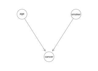
You see there are three circles representing the three variables, and the arrows designate that the cancer variable is conditioned by smoker and age. That's it. That's a PGM. A PGM is simply a fancy name for conditional probability with a graphical representation.
Don't be deceived by the simplicity: that's one of the strengths of the technique. The graphical representation makes it very easy to understand what would be incomprehensible as a collection of probability tables. For example, here's a picture of a large PGM used to diagnose liver disorders:

from A Bayesian Network Model for Diagnosis of Liver Disorders
Now, PGMs have a few unique strengths over classical modelling techniques like regression. I'm going to list them here, and then we'll spend the rest of the post building one (in R), and demonstrating each of these advantages:
- Simple graphical representation makes them easy to comprehend
- Predictions are omni-directional: there is no independent/dependent variable distinction
- Allows for chains of causal relationships between variables
- Easily incorporates both domain knowledge and raw data
- Missing values are no problem
- They can easily be made dynamic by connecting to underlying data [we won't be doing this]
And, yes, I did say we're going to be using R today. I know, I know: Python is so much nicer. In the case of PGMs, however, the R libraries are just a lot friendlier and better maintained.
One brief aside: whenever I set out to understand a new machine learning technique, I feel like my first task is to demystify the jargon. Probabilistic graphical models are also widely called Bayesian networks. I don't think Bayesian network is a very good name because I don't think it offers any clues as to what we're talking about. Hopefully you can see what the probabilistic and the graphical in PGM refer to now.
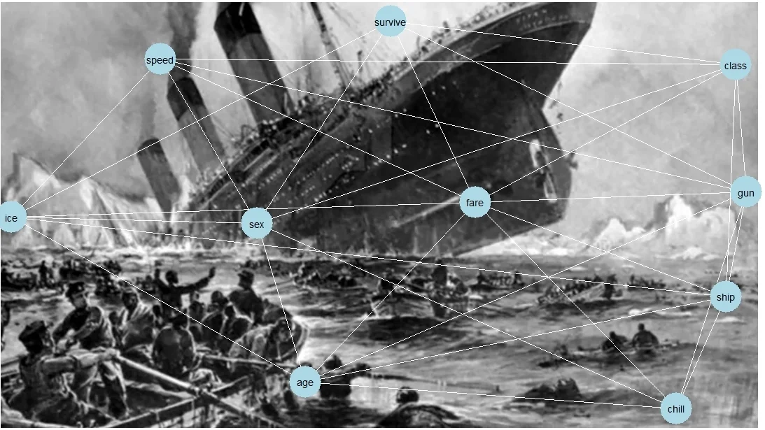
We're going to start by building a simple PGM to predict the likelihood of surviving the sinking of the Titanic given a passenger's gender and class. We're using the standard Titanic dataset which is widely available (eg. on Kaggle). It's well known that gender & class were strong determinants of a passenger's chance of survival.
## import Titanic data
FileLoc = "c:\\folder\\folder\\"
FileName = 'titanic.txt'
File = paste(FileLoc,FileName,sep="")
titanic.df <-read.delim(File,header=TRUE,sep="\t", stringsAsFactors=FALSE)

## drop any nulls
titanic.df = titanic.df[complete.cases(titanic.df[,c('survived','pclass','sex','fare')]),]

## define variables as factors
titanic.df$survived = as.factor(titanic.df$survived)
titanic.df$sex = as.factor(titanic.df$sex)
titanic.df$pclass = as.factor(titanic.df$pclass)

head(titanic.df[,c('survived','pclass','sex')])
##   survived pclass    sex
## 1        0      3   male
## 2        1      1 female
## 3        1      3 female
## 4        1      1 female
## 5        0      3   male
## 6        0      3   male
That's what it looks like. Let's take a look at the proportion of survivors given gender & class:
xtabs(survived~pclass+sex,
      setNames(aggregate(data=titanic.df,
                         as.numeric(as.character(survived))~sex+pclass, FUN=mean),
               c('sex','pclass','survived')))
##       sex
## pclass    female      male
##      1 0.9680851 0.3688525
##      2 0.9210526 0.1574074
##      3 0.5000000 0.1354467
Basically:
- Women were more likely to survive than men
- Survival rates were highest amongst first class passengers, then second. Third class had the lowest survival rates.
Now we'll fit a PGM to it with the bnlearn package.
#install.packages('bnlearn')
library(bnlearn)

#source("http://bioconductor.org/biocLite.R")
#biocLite("Rgraphviz")

# create an empty PGM skeleton
res = empty.graph(names(titanic.df[,c('survived','pclass','sex')]))

# define probabilistic relationships to encode
modelstring(res) = "[pclass][sex][survived|pclass:sex]"

# fit to dataset
titanic.bn <- bn.fit(res, data=titanic.df[,c('survived','pclass','sex')])

# what does our PGM look like?
graphviz.plot(titanic.bn)

In the argot of graph theory, the variables are variously known as nodes or vertices. The arrows are called arcs or edges.
You'll notice that I've specified the causal relationship between the three variables with the modelstring statement. There are algorithms designed to figure that out and, well, they're rather complicated. It's beyond the scope of today's post. I'll also mention that, to keep it simple, we'll be using discrete variables only. PGMs are perfectly happy using continuous variables - you just need to specify the distributions.
Now, we can ask R to print out the probabilities at each node:
titanic.bn
##
##   Bayesian network parameters
##
##   Parameters of node survived (multinomial distribution)
##
## Conditional probability table:
##
## , , sex = female
##
##         pclass
## survived          1          2          3
##        0 0.03191489 0.07894737 0.50000000
##        1 0.96808511 0.92105263 0.50000000
##
## , , sex = male
##
##         pclass
## survived          1          2          3
##        0 0.63114754 0.84259259 0.86455331
##        1 0.36885246 0.15740741 0.13544669
##
##
##   Parameters of node pclass (multinomial distribution)
##
## Conditional probability table:
##
##         1         2         3
## 0.2424242 0.2065095 0.5510662
##
##   Parameters of node sex (multinomial distribution)
##
## Conditional probability table:
##
##   female     male
## 0.352413 0.647587
Now we have our model, we can ask it to make some predictions:
# Prob survived
cpquery(titanic.bn, (survived==1), TRUE)
## [1] 0.3654
# Prob survived given female, class 1
cpquery(titanic.bn, (survived==1), (sex=='female' & pclass==1))
## [1] 0.9661017
# Prob survived given male, class 3
cpquery(titanic.bn, (survived==1), (sex=='male' & pclass==3))
## [1] 0.1292479
The sharp reader would have noted that the results from bnlearn differ slightly from the raw probability table we calculated above. This is because, by default, cpquery estimates results using sampling.
So far, nothing special. Let's start to look at some of those advantages I listed at the start of the post.
Missing values are no problem: I can make predictions even if I don't have values for some variables. (This is done simply by summing across the unobserved conditions).
# Prob survived given class 3, gender unknown
cpquery(titanic.bn, (survived==1), (pclass==3))
## [1] 0.2877055
# Prob survived given male, class unknown
cpquery(titanic.bn, (survived==1), (sex=='male'))
## [1] 0.1945231
Omnidirectional: predictions can (usually) be made for any variable, given any other variable(s): if we have a regression model, we are only predicting the independent variable. With a PGM, I can treat any variables as 'evidence' to predict any other variables:
# What if we want to know the probability of a survivor being male?
cpquery(titanic.bn, (sex=='male'), (survived==1))
## [1] 0.3593407
# What if we want to know the probability of a female victim being 1st class?
cpquery(titanic.bn, (pclass==1), (survived==0 & sex=='female'))
## [1] 0.03448276
When we use evidence to explain or predict an outcome it is called causal reasoning. For example, using symptoms to diagnose an illness. We can also go the other way: given an outcome, look back at the causes or explanations. This is called evidential reasoning. For example, given an illness, what were the symptoms? PGMs are neat in that they can easily go in both directions. This makes PGMs very good for predicting so-called "hidden" (unobserved) variables or constructs which might sit between a number of evidence and outcome variables.
It's worth knowing that we can ask bnlearn to give us a distribution:
# What is class distribution of survivors:
prop.table(table(cpdist(titanic.bn, 'pclass', (survived==1))))
##
##         1         2         3
## 0.3694843 0.2291334 0.4013822
So far, so good. But the best is yet to come. Unlike, say, logistic regression, we aren't limited to a single causal relationship between one independent variable and lots of dependent ones. With a PGM, we can have chains of causality.
For example, we have a varaible for the class of a passenger. We would expect this to be a function of the fare that they paid. Let's extend our network so that class is conditioned by fare.
Unfortunately, bnlearn doens't allow us to do this directly. But it is trivial to fit a new network to the parameters of our existing one plus the new variable.
# Determine a simple relationship between fare and class
# Break fare into two categories cutting at $30
titanic.df$c_fare <- ifelse(titanic.df$fare > 30, c("expensive"), c("cheap"))

## define fare variable
# specify probability of fare values
pfare = matrix(table(titanic.df$c_fare) / nrow(titanic.df),
               ncol=2, dimnames=list(NULL, c("cheap", "expensive")))

print(pfare)
##          cheap expensive
## [1,] 0.7373737 0.2626263
# specify probability conditional matrix of class|fare
class_given_fare = prop.table(table(titanic.df$pclass,titanic.df$c_fare), 2)
dim(class_given_fare) = c(3, 2)
dimnames(class_given_fare) = list("pclass" =  c(1, 2, 3),
                                 "fare" = c("cheap", "expensive"))

print(class_given_fare)
##       fare
## pclass      cheap  expensive
##      1 0.07153729 0.72222222
##      2 0.24353120 0.10256410
##      3 0.68493151 0.17521368
# create new PGM
res2 = empty.graph(c('survived','pclass','sex','fare'))
modelstring(res2) = "[sex][fare][pclass|fare][survived|pclass:sex]"

# fit model
titanic.bn2 <- custom.fit(res2, dist=list(sex=titanic.bn$sex$prob,
                                          pclass=class_given_fare,
                                          survived=titanic.bn$survived$prob,
                                          fare=pfare))

graphviz.plot(titanic.bn2)

There it is. Now, let's imagine that we don't know what class a passenger is travelling, but we know their fare. We can still make a prediction about their chances of survival.
cpquery(titanic.bn2, (survived==1), (fare=='expensive'))
## [1] 0.504126
This brings me to the last strength I wish to highlight: that PGMs make it easy to incorporate domain knowledge. Domain knowledge can take the form of specifying the causal relationships between variables (the 'arrows'), as well as the probability tables at each node. Domain knowledge is often subjective and, yes, it is a strength of PGMs that they can incorporate subjective knowledge. There's not much room for it in, say, a random forest or many other machine learning techniques. A PGM can be built from a mixture of objective data and subjective beliefs. You can also find PGMs that have been built entirely from expert opinions.
Let's work through an example of incorporating a wholly unsubstantiated opinion into our model. We just saw that it's very easy to tinker with a PGM. In the example of the fare variable, we inserted a node into the PGM by simply supplying the necessary probability tables. We derived that probability table from raw data - but we didn't have to. What if we had additional domain knowledge from other sources? In fact, we do: from the film, Titanic.
In James Cameron's Titanic, it isn't class that determines your fate, but whether or not you are an entitled asshole. According to James Cameron's God, entitled assholes are more deserving of death. Now, as cliché has it, there's a strong correlation between class and the poessession of a repulsive sense of entitlement, but it's not a perfect correlation (take the exception of Rose, for example).
Let's add this knowledge to our PGM. We'll create a new variable - entitlement - which is conditioned by class and which, in turn, conditions survival.
# P(entitlement | class)
entitlement_given_class <- matrix(c(0.7, 0.3, 0.5, 0.5, 0.3, 0.7),
                                  ncol=3, dimnames=list("entitlement" = c("yes", "no"),
                                                        "pclass" =  c(1, 2, 3)))

print(entitlement_given_class)
##            pclass
## entitlement   1   2   3
##         yes 0.7 0.5 0.3
##         no  0.3 0.5 0.7
# P(surived | entitlement, sex)
# this is a 3d matrix
survived_given_entitlement <- c(0.6, 0.4, 0.4, 0.6, 0.8, 0.2, 0.7, 0.3)
dim(survived_given_entitlement) <- c(2, 2, 2)
dimnames(survived_given_entitlement) <- list("survived"=c(0,1), "entitlement"=c('yes','no'), "sex"=c('female','male'))
print(survived_given_entitlement)
## , , sex = female
##
##         entitlement
## survived yes  no
##        0 0.6 0.4
##        1 0.4 0.6
##
## , , sex = male
##
##         entitlement
## survived yes  no
##        0 0.8 0.7
##        1 0.2 0.3
# Rebuild PGM with new structure
res3 = empty.graph(c('survived','pclass','sex','fare','entitlement'))
modelstring(res3) = "[sex][fare][pclass|fare][entitlement|pclass][survived|entitlement:sex]"
titanic.bn3 <- custom.fit(res3, dist=list(sex=titanic.bn2$sex$prob,
                                          fare=titanic.bn2$fare$prob,
                                          pclass=titanic.bn2$pclass$prob,
                                          entitlement=entitlement_given_class,
                                          survived=survived_given_entitlement))

graphviz.plot(titanic.bn3)

Let's go ahead and use our model:
# query: if entitled, what are survival chances?
cpquery(titanic.bn3, (survived==1), (entitlement=='yes'))
## [1] 0.2638376
# if fare was expensive, what is chance of being entitled?
cpquery(titanic.bn3, (entitlement=='yes'), (fare=='expensive'))
## [1] 0.626646
# if died and male, what is chance of being entitled?
cpquery(titanic.bn3, (entitlement=='yes'), (survived==1 & sex=='male'))
## [1] 0.3115578
That's about all I wanted to explore today.
There is, of course, a vast literature on PGMs and I've only scratched the surface. Things get much more complicated if you want to, say, automatically infer the network from the data. In fact, things get much more complicated if you just want to use continuous variables. Here's a couple of lucid resources:
- The
bnlearnpackages was the simplest, clearest implementation I found. The author, Marco Scutari, has also written a couple of welcoming and approachable books. See www.bnlearn.com - Stanford has a Coursera subject on PGMs. It doesn't look like it's every going to run again, but all the materials are online. If you're looking for an academic (read: dense, abstract, symbolic) introduction, then this is very good.
PGMs have proved especially good at assisting reasoning where there are a large number of variables and outcomes to consider, not all of which might be observed. They show particular promise for making medical diagnoses.
Let's finish with a fun, celebrated example of PGMs: Microsoft's primitive virtual Office assistant, Clippy. This 1998 paper by MS's Decision Theory & Adaptive Systems Group makes for interesting reading: The Lumiere Project: Bayesian User Modeling for Inferring the Goals and Needs of Software Users.

They say that understanding breeds empathy and, by gosh, having looked at Clippy from his creator's perspective I do have a touch of sympathy for that most irritating animated piece of disposable stationery.
That's it. Next post we'll be returning to beloved Python to look at so-called “deep learning” and convolutional neural networks.