
Today we're going to look at a recent innovation in neural networks called an autoencoder. Autoencoders are unsupervised neural networks that can automatically abstract useful features from data. We'll see how they can take images of handwritten numbers and abstract basic visual features like horizontal and vertical penstrokes, arcs and circles, and so forth. Once we've coded and fit an autoencoder - pausing briefly to understand the sparsity constraint - then we'll visualise what it has learned.
Aside on background knowledge: In this post, we're going to be looking at a variation on the archetypal neural network. Neural nets are complicated enough to have entire university computer science subjects dedicated to them. Explaining the fundamental nuts and bolts of neural nets is not the purpose of this post, and I hope that such background knowledge isn't necessary to get the conceptual gist :-) I want to focus on what the autoencoder does, how it works and its unique points of difference from a basic neural net. For those who want to get into the detail of neural nets, I highly recommend starting with two resources: the well-illustrated and practical online notes for Stanford class CS231n: Convolutional Neural Networks for Visual Recognition and the very lucid Coursera Machine Learning course by Professor Andrew Ng.
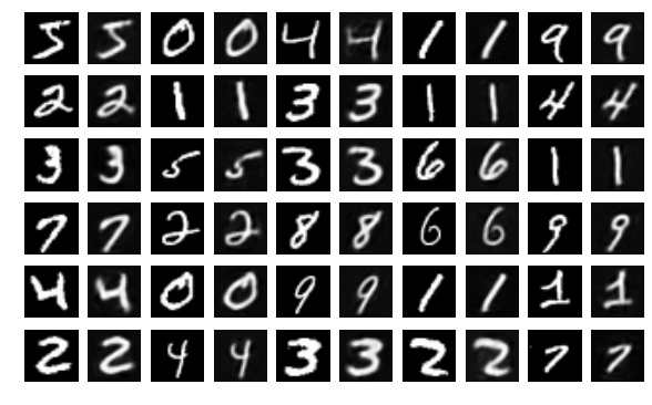
Here is a machine learning problem: we have some images of handwritten digits:

One thing we might want to do is teach a computer to recognise and differentiate between them.
Now, here is one of those figures in raw form (as the computer "sees" it):
0.0, 0.0, 0.0, 0.0, 0.0, 0.0, 0.0, 0.0, 0.0, 0.0, 0.0, 0.0, 0.0, 0.0, 0.0, 0.0, 0.0, 0.0, 0.0, 0.0, 0.0, 0.0, 0.0, 0.0, 0.0, 0.0, 0.0, 0.0, 0.0, 0.0, 0.0, 0.0, 0.0, 0.0, 0.0, 0.0, 0.0, 0.0, 0.0, 0.0, 0.0, 0.0, 0.0, 0.0, 0.0, 0.0, 0.0, 0.0, 0.0, 0.0, 0.0, 0.0, 0.0, 0.0, 0.0, 0.0, 0.0, 0.0, 0.0, 0.0, 0.0, 0.0, 0.0, 0.0, 0.0, 0.0, 0.0, 0.0, 0.0, 0.0, 0.0, 0.0, 0.0, 0.0, 0.0, 0.0, 0.0, 0.0, 0.0, 0.0, 0.0, 0.0, 0.0, 0.0, 0.0, 0.0, 0.0, 0.0, 0.0, 0.0, 0.0, 0.0, 0.0, 0.0, 0.0, 0.0, 0.0, 0.0, 0.0, 0.0, 0.0, 0.0, 0.0, 0.0, 0.0, 0.0, 0.0, 0.0, 0.0, 0.0, 0.0, 0.0, 0.0, 0.0, 0.0, 0.0, 0.0, 0.0, 0.0, 0.0, 0.0, 0.0, 0.0, 0.0, 0.0, 0.0, 0.0, 0.0, 0.0, 0.0, 0.0, 0.0, 0.0, 0.0, 0.0, 0.0, 0.0, 0.0, 0.0, 0.0, 0.0, 0.0, 0.0, 0.0, 0.0, 0.0, 0.0, 0.0, 0.0, 0.0, 0.0, 0.0, 0.01, 0.07, 0.07, 0.07, 0.49, 0.53, 0.69, 0.1, 0.65, 1.0, 0.97, 0.5, 0.0, 0.0, 0.0, 0.0, 0.0, 0.0, 0.0, 0.0, 0.0, 0.0, 0.0, 0.0, 0.12, 0.14, 0.37, 0.6, 0.67, 0.99, 0.99, 0.99, 0.99, 0.99, 0.88, 0.67, 0.99, 0.95, 0.76, 0.25, 0.0, 0.0, 0.0, 0.0, 0.0, 0.0, 0.0, 0.0, 0.0, 0.0, 0.0, 0.19, 0.93, 0.99, 0.99, 0.99, 0.99, 0.99, 0.99, 0.99, 0.99, 0.98, 0.36, 0.32, 0.32, 0.22, 0.15, 0.0, 0.0, 0.0, 0.0, 0.0, 0.0, 0.0, 0.0, 0.0, 0.0, 0.0, 0.0, 0.07, 0.86, 0.99, 0.99, 0.99, 0.99, 0.99, 0.78, 0.71, 0.97, 0.95, 0.0, 0.0, 0.0, 0.0, 0.0, 0.0, 0.0, 0.0, 0.0, 0.0, 0.0, 0.0, 0.0, 0.0, 0.0, 0.0, 0.0, 0.0, 0.31, 0.61, 0.42, 0.99, 0.99, 0.8, 0.04, 0.0, 0.17, 0.6, 0.0, 0.0, 0.0, 0.0, 0.0, 0.0, 0.0, 0.0, 0.0, 0.0, 0.0, 0.0, 0.0, 0.0, 0.0, 0.0, 0.0, 0.0, 0.0, 0.05, 0.0, 0.6, 0.99, 0.35, 0.0, 0.0, 0.0, 0.0, 0.0, 0.0, 0.0, 0.0, 0.0, 0.0, 0.0, 0.0, 0.0, 0.0, 0.0, 0.0, 0.0, 0.0, 0.0, 0.0, 0.0, 0.0, 0.0, 0.0, 0.0, 0.55, 0.99, 0.75, 0.01, 0.0, 0.0, 0.0, 0.0, 0.0, 0.0, 0.0, 0.0, 0.0, 0.0, 0.0, 0.0, 0.0, 0.0, 0.0, 0.0, 0.0, 0.0, 0.0, 0.0, 0.0, 0.0, 0.0, 0.0, 0.04, 0.75, 0.99, 0.27, 0.0, 0.0, 0.0, 0.0, 0.0, 0.0, 0.0, 0.0, 0.0, 0.0, 0.0, 0.0, 0.0, 0.0, 0.0, 0.0, 0.0, 0.0, 0.0, 0.0, 0.0, 0.0, 0.0, 0.0, 0.0, 0.14, 0.95, 0.88, 0.63, 0.42, 0.0, 0.0, 0.0, 0.0, 0.0, 0.0, 0.0, 0.0, 0.0, 0.0, 0.0, 0.0, 0.0, 0.0, 0.0, 0.0, 0.0, 0.0, 0.0, 0.0, 0.0, 0.0, 0.0, 0.0, 0.32, 0.94, 0.99, 0.99, 0.47, 0.1, 0.0, 0.0, 0.0, 0.0, 0.0, 0.0, 0.0, 0.0, 0.0, 0.0, 0.0, 0.0, 0.0, 0.0, 0.0, 0.0, 0.0, 0.0, 0.0, 0.0, 0.0, 0.0, 0.0, 0.18, 0.73, 0.99, 0.99, 0.59, 0.11, 0.0, 0.0, 0.0, 0.0, 0.0, 0.0, 0.0, 0.0, 0.0, 0.0, 0.0, 0.0, 0.0, 0.0, 0.0, 0.0, 0.0, 0.0, 0.0, 0.0, 0.0, 0.0, 0.0, 0.06, 0.36, 0.99, 0.99, 0.73, 0.0, 0.0, 0.0, 0.0, 0.0, 0.0, 0.0, 0.0, 0.0, 0.0, 0.0, 0.0, 0.0, 0.0, 0.0, 0.0, 0.0, 0.0, 0.0, 0.0, 0.0, 0.0, 0.0, 0.0, 0.0, 0.98, 0.99, 0.98, 0.25, 0.0, 0.0, 0.0, 0.0, 0.0, 0.0, 0.0, 0.0, 0.0, 0.0, 0.0, 0.0, 0.0, 0.0, 0.0, 0.0, 0.0, 0.0, 0.0, 0.0, 0.0, 0.18, 0.51, 0.72, 0.99, 0.99, 0.81, 0.01, 0.0, 0.0, 0.0, 0.0, 0.0, 0.0, 0.0, 0.0, 0.0, 0.0, 0.0, 0.0, 0.0, 0.0, 0.0, 0.0, 0.0, 0.0, 0.0, 0.15, 0.58, 0.9, 0.99, 0.99, 0.99, 0.98, 0.71, 0.0, 0.0, 0.0, 0.0, 0.0, 0.0, 0.0, 0.0, 0.0, 0.0, 0.0, 0.0, 0.0, 0.0, 0.0, 0.0, 0.0, 0.0, 0.09, 0.45, 0.87, 0.99, 0.99, 0.99, 0.99, 0.79, 0.31, 0.0, 0.0, 0.0, 0.0, 0.0, 0.0, 0.0, 0.0, 0.0, 0.0, 0.0, 0.0, 0.0, 0.0, 0.0, 0.0, 0.0, 0.09, 0.26, 0.84, 0.99, 0.99, 0.99, 0.99, 0.78, 0.32, 0.01, 0.0, 0.0, 0.0, 0.0, 0.0, 0.0, 0.0, 0.0, 0.0, 0.0, 0.0, 0.0, 0.0, 0.0, 0.0, 0.0, 0.07, 0.67, 0.86, 0.99, 0.99, 0.99, 0.99, 0.76, 0.31, 0.04, 0.0, 0.0, 0.0, 0.0, 0.0, 0.0, 0.0, 0.0, 0.0, 0.0, 0.0, 0.0, 0.0, 0.0, 0.0, 0.0, 0.22, 0.67, 0.89, 0.99, 0.99, 0.99, 0.99, 0.96, 0.52, 0.04, 0.0, 0.0, 0.0, 0.0, 0.0, 0.0, 0.0, 0.0, 0.0, 0.0, 0.0, 0.0, 0.0, 0.0, 0.0, 0.0, 0.0, 0.0, 0.53, 0.99, 0.99, 0.99, 0.83, 0.53, 0.52, 0.06, 0.0, 0.0, 0.0, 0.0, 0.0, 0.0, 0.0, 0.0, 0.0, 0.0, 0.0, 0.0, 0.0, 0.0, 0.0, 0.0, 0.0, 0.0, 0.0, 0.0, 0.0, 0.0, 0.0, 0.0, 0.0, 0.0, 0.0, 0.0, 0.0, 0.0, 0.0, 0.0, 0.0, 0.0, 0.0, 0.0, 0.0, 0.0, 0.0, 0.0, 0.0, 0.0, 0.0, 0.0, 0.0, 0.0, 0.0, 0.0, 0.0, 0.0, 0.0, 0.0, 0.0, 0.0, 0.0, 0.0, 0.0, 0.0, 0.0, 0.0, 0.0, 0.0, 0.0, 0.0, 0.0, 0.0, 0.0, 0.0, 0.0, 0.0, 0.0, 0.0, 0.0, 0.0, 0.0, 0.0, 0.0, 0.0, 0.0, 0.0, 0.0, 0.0, 0.0, 0.0, 0.0, 0.0, 0.0, 0.0, 0.0, 0.0, 0.0, 0.0, 0.0, 0.0, 0.0, 0.0, 0.0, 0.0, 0.0, 0.0
Do you know which one it is? Of course not. (It's the very first one: the 5). To the computer, each 28x28 pixel image is a list of 784 values ranging between 0 (black) and 1 (white).
How do we humans tell one number from another? It's not a trick question: we recognise that each figure is comprised of a certain arrangement of vertical strokes, horizontal strokes, arcs and circles. Now: how can we teach a computer to differentiate figures? Well, if the computer could "see" the same component visual features that we could then it would be easy: two stacked circles is an '8', one large circle is a '0', and so. But the computer can't "see" those features - to it, each image is only an unhelpful, long list of 784 values.

What we're talking about are features. If we want to teach the computer to distinguish handwritten numbers then we need to give it features which are relevant to the task. Not 784 raw values, but features like, "Is there a vertical stroke present?" or, "Are there any circles?"
How can the computer get features from image data? In many machine learning tasks, we might create features manually using our own expertise: for example, we might take the logarithm of one variable or the ratio between two others. Let's dispel that idea right away. Consider all the possible ways that people write 5:
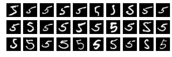
When there is so much variation, how could we possibly create manual rules that would parse the huge list of values that comprise an image and return "circle present" or "two horizontal strokes?" (And this is a very simple example: consider the problem of teaching a computer to recognise faces or objects).
For a long time, the efforts of the computer vision community were directed towards finding some complicated rules which would surface useful, generalised features. You can understand why progress was slow. The breakthrough was quite ingenious: teach the computer to discover the features for itself.
Autoencoders
An autoencoder is a type of neural network but with two special differences. The first is that it is trained to reconstruct its own input but with reduced dimensionality. Huh? That won't make much sense the first time you read it, so let's unpack it. A picture:

Let's apply this diagram to our images of handwritten digits. The images are each 28x28 pixels, which means 784 values are going into the input layer. That's one input per pixel. The output layer will also have 784 neurons, which correspond to the same pixels. The network is trained so that each output neuron is trying to predict the pixel value of the corresponding input. In symbolic terms, if we say our autoencoder is a mathematical function $h$, then we want it to learn $h$ so that $h(x) = x$.
Now, this would seem to be a trivial and pointless thing to learn, except there's the catch: the hidden layer has far less than 784 neurons (today we're going to use 200). This means that the network cannot learn an exact representation of all 784 pixels in the image - it is forced to learn a reduced dimensional representation, and in doing so it will seek common features that can explain variance. In the case of handwritten digits, these will be the basic penstrokes. (It may help some readers to recognise that this is the neural network equivalent to principal components analysis.)
The second way that autoencoders differ from typical, supervised neural nets is that we enforce an additional constraint called sparsity. I'll explain this below as we get into the code.
Coding an autoencoder
Let's look at an implementation in Python 2.7. This is a rudimentary autoencoder with no bells or whistles. I've broken the code into parts:
- Import and preprocess data
- Set parameters and define autoencoder backpropagation function
- Run optimise process to train autoencoder
- Visualise what it has learned
So, let's bring in our dataset. The MNIST database of handwritten digits is a near legendary dataset for machine learning. It's appeared in countless papers and competitions. You can download it in convenient Python pickle format from here. Once we've imported it, we'll standardise it and scale it to the range of [0.1,0.9] which is best for a sigmoid activation function.
Now we'll code our autoencoder. The next code block begins with defining some parameters and hyperparameters, and then defines the backpropagation function which will train the autoencoder.
It should seem straightforward to those familiar with neural nets, with the exception of one surprise: the sparsity constraint. This is an additional penalty employed in autoencoders which doesn't appear in basic neural networks. Conceptually, the purpose is to constrain the amount of activity permitted in the hidden layer and prevent the network from simply learning a copy of the input data (eg. the identity function). The network is instead forced to find common features within the data. I'll explain how it works.
Firstly, we're employing the typical sigmoid activation function in our network, so the activation (output) of any neuron will always be between 0 and 1. A reminder that sigmoid is:
$$a(x)=\frac{1}{(1+e^{-x})}$$
Therefore, the mean activation across all the neurons in the hidden layer will also be between 0 and 1. We will call the mean activation across the hidden layer $\hat{\rho}$ ("rho hat") and calculate it as:
$$\hat{\rho} = \frac{1}{N}\sum a(x_i)$$
Where $N$ is the number of observations. You will see this in the code as rho_hat = np.sum(hidden_layer, axis = 1) / N
Now we specify the sparsity parameter $\rho$ ("rho"), which represents the average activation we would like to have in the hidden layer. In other words, we would like $\rho \approx \hat{\rho}$. Today we'll be setting $\rho = 0.1$. To meet that constraint, clearly most of the neurons in the hidden layer are going to need to be relatively inactive and outputting near zero.
To achieve this, we add an additional term to our cost function that penalises the network if $\rho$ and $\rho = \hat{\rho}$ diverge:
$$\sum \rho \log \frac{\rho}{\hat{\rho}} + (1-\rho) \log \frac{1-\rho}{1-\hat{\rho}}$$
This penalty gets larger the more than $\hat{\rho}$ (the average activation) diverges from $\rho$. For additional control, we throw in one extra hyperparameter $\beta$ which we can manipulate to boost or diminish the impact of sparsity.
In the code: cost_sparsity = beta * np.sum(rho * np.log(rho / rho_hat) + (1 - rho) * np.log((1 - rho) / (1 - rho_hat)))
There is also, of course, an adjustment to be made to our backpropagation gradient calculations. I won't write it out here but you can see it in the code.
Everything is defined: now we just throw it into the SciPy's minimisation algorithm, which will perform gradient descent to seek the set of weights with the lowest error:
We've (hopefully) succeeded in training our autoencoder. Now for the interesting part: let's see what the network has learned. Since our dataset is images, we can do this by simply visualising the weights associated with the hidden layer:

Here we can see the visual features which the autoencoder has learned: the strokes and arcs which make up the handwritten digits. Each neuron has learned to detect a certain visual feature (they are sometimes referred to as "edge detectors"). Admittedly there are some neurons that seem to have learned features that are over-specific to certain numbers (I can see a few 8s), and there are many neurons that have learned slight variations on a theme (the many slightly different angled vertical strokes).
Although we aren't really interested in the output of the autoencoder, it is still interesting to visualise how close it is to the input images:
Even though the autoencoder is constrained to use only 200 hidden neurons, it manages outputs that are very similar to the original images. This means that we don't need 784 bits of information to store a recognisible digit: they are perfectly recognisable using only 200 bits of information (and possibly less).
Now that we've trained the autoencoder, what can we do with it? We can feed images through it and it will detect the presence of these visual features. The outputs of the autoencoder's hidden layer can be fed directly into other machine learning techniques. So, instead of trying to learn from the 784 pixels that make up each image, we can learn from the 200 outputs of our autoencoder, each of which will correspond to meaningful visual features (strokes, arcs, circles, etc).
And although it has been trained on handwritten digits, we could feed other sorts of images through it. For example, we might feed images of letters to it and have it tell us whether these types of penstrokes are present. In this way, our autoencoder has abstracted useful visual features which can be generalised.
Postscript: deep learning & stacked autoencoders
The autoencoder is one of a handful of advances in neural networks which are collectively referred to as deep learning. Deep learning approaches have lead to breakthroughs in computer vision and speech recognition, and power services like Facebook's face recognition and Siri. Deep learning has been so successful that it has even graduated to mainstream buzz with press articles like 'Deep Learning' Will Soon Give Us Super-Smart Robots (Wired) and Google develops computer program capable of learning tasks independently (the Guardian). Here's a typical sentence from the Guardian's article: "The agent uses a method called 'deep learning' to turn the basic visual input into meaningful concepts, mirroring the way the human brain takes raw sensory information and transforms it into a rich understanding of the world."
So what is it? "Deep learning" is often used in a vague, hand-wavy way to mean "really big neural networks." But I think we're really talking about three developments in neural networks which have made them much more effective:
- Massive increases in computing power enabling much bigger networks trained on much larger datasets. (This is obvious and not terribly interesting). Reportedly, the neural network that powers the image classification in Google Photos is 13 layers deep.
- Development of strategies for generalising learning: Facial recognition is made difficult because faces can appear in images near or far, in different locations, in profile or rotated in different directions, etc. Accents present a similar problem for speech recognition. A variety of interesting strategies have been proposed to counter these problems, a good example of which is the convolutional neural network.
- Development of strategies for abstracting meaningful features from data
It's the third point we've been discussing today. In large deep learning neural networks, there would be a hierarchy of autoencoder-like layers, each of which abstracts higher level features from previous layers. For example, the lowest layer would detect edges (like our autoencoder), the second layer might use combinations of edges to detect shapes, the third layer could combine the shapes into objects, and so on. By the final layers, features are being combined into meaningful objects.
We understand that the human perceptual systems operate in a similar fashion - with a hierarchy of increasingly complex feature detectors. Since our perceptual systems are frankly amazing, it makes sense to design machine learning systems that mimic them.