Understanding machine learning techniques by visualising their decision boundaries

At work, I sometimes find myself trying to explain the difference between different modelling or machine learning techniques. For example, the difference between regression models and decision trees. But simply explaining how they work algorithmically rarely gives somebody that satisfying feeling of intuition that is the product of understanding.

Seeking to understand, people will often ask when one technique works better than another. This is a good question and it helps to see how different techniques perform on different problems. One way to visualise this is to compare plots of decision boundaries. Given a supervised learning problem where there are points of two classes (let's say red and blue), we can train machine learning techniques to predict which class a hypothetical point should belong to.

Here's an example produced by a little Python script I whipped up. In the first plot is a randomly generated problem - a two-dimensional space with red and blue points. We then train a variety of machine learning techniques on that problem. Their task is to discriminate between the red and blue points. We can illustrate their solution by colouring the space red or blue depending on what class they predict that region belongs to.

To reiterate, the space is coloured according to whether the machine learning technique predicts it belongs to the red or the blue class. (For some techniques, we can use shade to represent their strength of belief in the colour of the region. For example, if a model predicts a high probability that a region is blue, then we shade that area darker blue). The line between coloured regions is called the decision boundary.

The first thing you might look for is how many points have been misclassified by being included in an incorrectly coloured region. To perfectly solve this problem, a very complicated decision boundary is required. The capacity of a technique to form really convoluted decision boundaries isn't necessarily a virtue, since it can lead to overfitting.

The main point of these plots, though, is to compare the decision boundaries that techniques are capable of. Looking at how different techniques try to solve the problem helps to develop an intuition of how they work. For example: regression, which must solve the problem using a linear equation, is only capable of continuous boundaries. Whereas decision trees, which proceed by bisecting continuous variables, can partition the space into isolated "blocks."

... and so on. Here's another example:

This problem illustrates the problem of overfitting. Simple, first-order linear regression is only capable of straight-line boundaries, whereas when we add interactions and polynomial terms then it can form curved boundaries. The straight-line solution of simple logistic regresion will almost certainly generalise better than the convoluted boundary produced when we add polynomial terms and interactions. Regularisation can address the problem of overfitting by constraining the polynomial & interaction coefficients and thus, visually speaking, limiting the flexibility of the boundary.

Here's another example, with a more difficult problem:

This problem is tricky because the red & blue classes are in opposing quadrants. Clearly, no straight line decision boundary is going to work and simple regression fails dismally. Problems where the classes form multiple clusters are often suited to k-Nearest Neighbours or tree based approaches.

Here's one last example of a difficult problem in which the blue points separate two groups of red points:

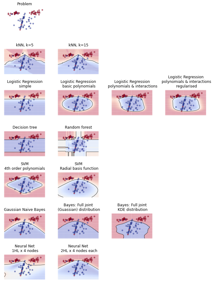
Here's the Python script I used to generate these plots. It's not the most elegant code, but it's clear and easy to tinker with. I run it in a Jupyter notebook. You can tweak the make_classification() function to generate different problems.

	### Prepeare python
	%pylab inline

	import numpy as np
	import pandas as pd
	import statsmodels.api as sm
	import scipy.stats as stats
	import neurolab as nl
	from sklearn.datasets import make_classification
	from sklearn import neighbors, tree, svm
	from sklearn.ensemble import RandomForestClassifier
	from sklearn.naive_bayes import GaussianNB


	### Helper functions for plotting
	# A function to plot observations on scatterplot
	def plotcases(ax):
	plt.scatter(xdf['x1'],xdf['x2'],c=xdf['y'], cmap=cm.coolwarm, axes=ax, alpha=0.6, s=20, lw=0.4)
	ax.spines['top'].set_visible(False)
	ax.spines['right'].set_visible(False)
	ax.spines['left'].set_visible(False)
	ax.spines['bottom'].set_visible(False)
	ax.tick_params(axis='both', which='both', left='off', right='off', top='off', bottom='off',
	labelleft='off', labelright='off', labeltop='off', labelbottom='off')

	# a function to draw decision boundary and colour the regions
	def plotboundary(ax, Z):
	ax.pcolormesh(xx, yy, Z, cmap=cm.coolwarm, alpha=0.1)
	ax.contour(xx, yy, Z, [0.5], linewidths=0.75, colors='k')


	### Generate train data
	X, y = make_classification(n_samples=100, n_features=2, n_informative=2, n_redundant=0, n_repeated=0,
	n_classes=2, n_clusters_per_class=2, weights=None, flip_y=0.02, class_sep=0.5,
	hypercube=True, shift=0.0, scale=0.5, shuffle=True, random_state=5)

	xdf = pd.DataFrame(X, columns=['x1','x2'])
	xdf['y'] = y


	### create plot canvas with 6x4 plots
	fig = plt.figure(figsize(12,16), dpi=1600)
	plt.subplots_adjust(hspace=.5)

	nrows = 7
	ncols = 4
	gridsize = (nrows, ncols)


	### 1. plot the problem ###
	ax0 = plt.subplot2grid(gridsize,[0,0])
	plotcases(ax0)
	ax0.title.set_text("Problem")

	# take boundaries from first plot and define mesh of points for plotting decision spaces
	x_min, x_max = plt.xlim()
	y_min, y_max = plt.ylim()
	nx, ny = 100, 100 # this sets the num of points in the mesh
	xx, yy = np.meshgrid(np.linspace(x_min, x_max, nx),
	np.linspace(y_min, y_max, ny))


	############# kNN #################
	### 2. kNN with k=5
	knn5 = neighbors.KNeighborsClassifier(n_neighbors=5)
	knn5.fit(xdf[['x1','x2']], xdf['y'])

	Z = knn5.predict_proba(np.c_[xx.ravel(), yy.ravel()])
	Z = Z[:,1].reshape(xx.shape)

	ax = plt.subplot2grid(gridsize, [1,0])
	ax.title.set_text("kNN, k=5")
	plotboundary(ax, Z)
	plotcases(ax)


	### 3. kNN with k=15
	knn15 = neighbors.KNeighborsClassifier(n_neighbors=15)
	knn15.fit(xdf[['x1','x2']], xdf['y'])

	Z = knn15.predict_proba(np.c_[xx.ravel(), yy.ravel()])
	Z = Z[:,1].reshape(xx.shape)

	ax = plt.subplot2grid(gridsize,[1,1])
	ax.title.set_text("kNN, k=15")
	plotboundary(ax, Z)
	plotcases(ax)


	########### logistic regression ##########
	### 4. Logistic regression - simple linear
	formula = ('y ~ x1 + x2')
	LRm = sm.GLM.from_formula(formula=formula, data=xdf, family=sm.families.Binomial()).fit()

	XX = pd.DataFrame((vstack([xx.ravel(), yy.ravel()]).T))
	XX.columns = xdf.columns[0:2]
	Z = LRm.predict(XX)
	Z = Z.reshape(xx.shape)

	ax = plt.subplot2grid(gridsize, [2,0])
	ax.title.set_text("Logistic Regression\n simple")
	plotboundary(ax, Z)
	plotcases(ax)


	### 5. Logistic regression - with basic polynomials
	formula = ('y ~ x1 + x2 + I(x12) + I(x22)')
	LRm = sm.GLM.from_formula(formula=formula, data=xdf, family=sm.families.Binomial()).fit()

	Z = LRm.predict(XX)
	Z = Z.reshape(xx.shape)

	ax = plt.subplot2grid(gridsize, [2,1])
	ax.title.set_text("Logistic Regression\n basic polynomials")
	plotboundary(ax, Z)
	plotcases(ax)


	### 6. Logistic regression - with polynomials & interactions
	formula = ('y ~ x1 + x2 + x1x2 + I(x12) + I(x22) + x1I(x1*2) + x2I(x2**2)\
	+ I(x13) + I(x23) + x1I(x13) + x2I(x2**3)')
	LRm = sm.GLM.from_formula(formula=formula, data=xdf, family=sm.families.Binomial()).fit()

	Z = LRm.predict(XX)
	Z = Z.reshape(xx.shape)

	ax = plt.subplot2grid(gridsize, [2,2])
	ax.title.set_text("Logistic Regression\n polynomials & interactions")
	plotboundary(ax, Z)
	plotcases(ax)


	### 7. Logistic regression - with polynomials & interactions, regularised
	# smaller alpha = weaker regularisation.
	formula = ('y ~ x1 + x2 + x1x2 + I(x12) + I(x22) + x1I(x1*2) + x2I(x2**2)\
	+ I(x13) + I(x23) + x1I(x13) + x2I(x2**3)')
	LRm = sm.Logit.from_formula(formula=formula, data=xdf).fit_regularized(alpha=0.5, maxiter = 200)

	Z = LRm.predict(XX)
	Z = Z.reshape(xx.shape)

	ax = plt.subplot2grid(gridsize, [2,3])
	ax.title.set_text("Logistic Regression\n polynomials & interactions\n regularised")
	plotboundary(ax, Z)
	plotcases(ax)



	##### TREE METHODS ########
	### 8. Decision tree
	dtree = tree.DecisionTreeClassifier()
	dtree = dtree.fit(xdf[['x1','x2']], xdf['y'])

	Z = dtree.predict_proba(np.c_[xx.ravel(), yy.ravel()])
	Z = Z[:,1].reshape(xx.shape)

	ax = plt.subplot2grid(gridsize, [3,0])
	ax.title.set_text("Decision tree")
	plotboundary(ax, Z)
	plotcases(ax)


	### 9. Random forest
	rf = RandomForestClassifier()
	rf.fit(xdf[['x1','x2']], xdf['y'])

	Z = rf.predict_proba(np.c_[xx.ravel(), yy.ravel()])
	Z = Z[:,1].reshape(xx.shape)

	ax = plt.subplot2grid(gridsize, [3,1])
	ax.title.set_text("Random forest")
	plotboundary(ax, Z)
	plotcases(ax)



	###### SUPPORT VECTOR MACHINES ###############
	## 10. SVM with 4th order polynomials
	svc2 = svm.SVC(kernel='poly',degree=4, probability=True)
	svc2.fit(xdf[['x1','x2']], xdf['y'])

	Z = svc2.predict_proba(np.c_[xx.ravel(), yy.ravel()])
	Z = Z[:,1].reshape(xx.shape)

	ax = plt.subplot2grid(gridsize, [4,0])
	ax.title.set_text("SVM\n4th order polynomials")
	plotboundary(ax, Z)
	plotcases(ax)



	## 11. SVM with radial basis function
	svc3 = svm.SVC(kernel='rbf', probability=True)
	svc3.fit(xdf[['x1','x2']], xdf['y'])

	Z = svc3.predict_proba(np.c_[xx.ravel(), yy.ravel()])
	Z = Z[:,1].reshape(xx.shape)

	ax = plt.subplot2grid(gridsize, [4,1])
	ax.title.set_text("SVM\n Radial basis function")
	plotboundary(ax, Z)
	plotcases(ax)


	####### Bayesian & Probabilistic methods ############
	### 12. Gaussian Naive Bayes
	gnb = GaussianNB()
	gnb.fit(xdf[['x1','x2']], xdf['y'])

	Z = gnb.predict_proba(np.c_[xx.ravel(), yy.ravel()])
	Z = Z[:,1].reshape(xx.shape)

	ax = plt.subplot2grid(gridsize, [5,0])
	ax.title.set_text("Gaussian Naive Bayes")
	plotboundary(ax, Z)
	plotcases(ax)


	### 13. Gaussian Bayes, non-naive (joint distribution)
	## Assumes multivariate normality
	# Specify prior: p(class). Assume that this is constant across all regions
	pClass1 = len(xdf[xdf['y']==1]) / float(len(xdf))
	pClass2 = len(xdf[xdf['y']==0]) / float(len(xdf))

	## Create likelihood distribution: p(datapoint \| class)
	## For each class, determine mean and variance across both variables
	# Collect means for both variables, for both classes
	Mux1C1 = xdf['x1'][xdf['y']==1].mean()
	Mux2C1 = xdf['x2'][xdf['y']==1].mean()
	Mux1C2 = xdf['x1'][xdf['y']==0].mean()
	Mux2C2 = xdf['x2'][xdf['y']==0].mean()

	# Collect vars for both variables, for both classes
	Varx1C1 = xdf['x1'][xdf['y']==1].std()
	Varx2C1 = xdf['x2'][xdf['y']==1].std()
	Varx1C2 = xdf['x1'][xdf['y']==0].std()
	Varx2C2 = xdf['x2'][xdf['y']==0].std()

	# use to create Normal distributions from these variables
	rangex1 = np.linspace(xdf['x1'].min(), xdf['x1'].max(), num=100)
	rangex2 = np.linspace(xdf['x2'].min(), xdf['x2'].max(), num=100)

	# generate Gaussian distributions for x1 and x2 within both class1 and class2
	C1x1 = np.array([stats.norm(Mux1C1, Varx1C1).pdf(i) for i in rangex1])
	C1x2 = np.array([stats.norm(Mux2C1, Varx2C1).pdf(i) for i in rangex2])
	C2x1 = np.array([stats.norm(Mux1C2, Varx1C2).pdf(i) for i in rangex1])
	C2x2 = np.array([stats.norm(Mux2C2, Varx2C2).pdf(i) for i in rangex2])

	# use this to create a joint likelihood distributions for class1 and class2:
	# These contain the joint probabilities for any given point whether it is in class1 or class2
	pLikelihoodC1Joint = np.dot(C1x2[:, None], C1x1[None, :])
	pLikelihoodC2Joint = np.dot(C2x2[:, None], C2x1[None, :])

	# Finally, put them together to create the two posterior distributions: p(class \| data)
	ScoreClass1GivenData = pLikelihoodC1Joint * pClass1 / (sum(pLikelihoodC1Joint * pClass1) + sum(pLikelihoodC2Joint * pClass2))
	ScoreClass2GivenData = pLikelihoodC2Joint * pClass2 / (sum(pLikelihoodC1Joint * pClass1) + sum(pLikelihoodC2Joint * pClass2))

	## for a given point, we calculate both likelihoods, and the max is the class we allocate to:
	# eg ScoreClass1GivenData > ScoreClass2GivenData
	Z = ScoreClass1GivenData > ScoreClass2GivenData
	Z = Z.reshape(xx.shape)

	ax = plt.subplot2grid(gridsize,[5,1])
	ax.title.set_text("Bayes: Full joint\n (Guassian) distribution")
	plotboundary(ax, Z)
	plotcases(ax)


	### 14. Bayes with joint, nonparametric (kernel density estimated) distributions
	## = Does NOT assume normality

	# Specify prior: p(class). [same as above]

	# Create likelihood distribution: p(datapoint \| class)
	# = estimate distribution using Kernel Density
	dens_1 = sm.nonparametric.KDEMultivariate(data=xdf[['x1','x2']][xdf['y']==0],
	var_type='cc', bw='normal_reference')

	dens_2 = sm.nonparametric.KDEMultivariate(data=xdf[['x1','x2']][xdf['y']==1],
	var_type='cc', bw='normal_reference')

	# generate distributions for x1 and x2 within both class1 and class2
	pLikelihoodC1Joint = dens_1.pdf(c_[xx.ravel(),yy.ravel()])
	pLikelihoodC2Joint = dens_2.pdf(c_[xx.ravel(),yy.ravel()])

	# Use Bayes rule to get posterior distribution, then convert back to matrix form
	ScoreClass1GivenData = pLikelihoodC1Joint * pClass1 / (sum(pLikelihoodC1Joint * pClass1) + sum(pLikelihoodC2Joint * pClass2))
	ScoreClass2GivenData = pLikelihoodC2Joint * pClass2 / (sum(pLikelihoodC1Joint * pClass1) + sum(pLikelihoodC2Joint * pClass2))

	ScoreClass1GivenData = ScoreClass1GivenData.reshape(xx.shape)
	ScoreClass2GivenData = ScoreClass2GivenData.reshape(xx.shape)

	# predict most likely class at each point on grid
	Z = ScoreClass1GivenData < ScoreClass2GivenData
	Z = Z.reshape(xx.shape)

	ax = plt.subplot2grid(gridsize, [5,2])
	ax.title.set_text("Bayes: Full joint\n KDE distribution")
	plotboundary(ax, Z)
	plotcases(ax)


	####### Neural Networks #########
	## Nb. these take a while to train & the neurolab library can be a bit tempramental
	## Can delete this chunk of code if desired
	yarr = np.matrix(y).T

	## Neural Net - 1HL, 3 hidden nodes
	net3 = nl.net.newff([[np.min( X[:,0]), np.max( X[:,0])], [np.min( X[:,1]), np.max( X[:,1])]], [4, 1])
	net3.trainf = nl.train.train_gd # use gradient descent, bfgs is too buggy in neurolab
	err = net3.train(X, yarr, show=100, goal=0.01)

	Z = net3.sim(np.vstack([xx.ravel(), yy.ravel()]).T)
	Z = Z.reshape(xx.shape)

	ax = plt.subplot2grid(gridsize,[6,0])
	ax.title.set_text("Neural Net\n 1HL x 4 nodes")
	plotboundary(ax, Z)
	plotcases(ax)


	## Neural Net - 2HL, 4 hidden nodes eacg
	net44 = nl.net.newff([[np.min( X[:,0]), np.max( X[:,0])], [np.min( X[:,1]), np.max( X[:,1])]], [4, 4, 1])
	net44.trainf = nl.train.train_gd # use gradient descent, bfgs is too buggy in neurolab
	err = net44.train(X, yarr, show=100, goal=0.01, lr=0.01)

	Z = net44.sim(np.vstack([xx.ravel(), yy.ravel()]).T)
	Z = Z.reshape(xx.shape)

	ax = plt.subplot2grid(gridsize,[6,1])
	ax.title.set_text("Neural Net\n 2HL x 4 nodes each")
	plotboundary(ax, Z)
	plotcases(ax)

view raw 20160215_Decision_boundaries.py hosted with ❤ by GitHub

2 Comments