
Convolutional neural networks are a type of neural network that have unique architecture especially suited to images. They have been spectacularly successful at image recognition, and now power services like the automated face tagging and object search in Google Photos.
In today's post I'll be talking about CNNs and training one to distinguish between images of cats and dogs. I'll be implementing the CNN in Google's TensorFlow deep learning software.
Cats are better
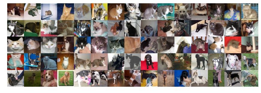
We’ve got 25,000 pictures of cats and dogs from Kaggle’s Dogs vs. Cats competition. This is what they look like:
Obviously, a computer can’t “see” a picture the way we do. To the computer, a colour picture is typically represented by a 3-dimensional array of numbers. All the pictures we’re using today are 64 pixels in height and 64 pixels in width, and then each pixel is defined by three integers: one each for the red, green, blue channels:

If you want to distinguish a cat from a dog, then you need to look at things like ears, whiskers, tails, tongues, fur textures, and so forth. These are the features that we (humans) use to discriminate. But none of these features are available to a computer, which knows only 12,288 independent integers (64x64x3).

At the pixel level, these two pictures are completely different. They would have virtually nothing in common. Yet they are unmistakably both dogs. And, again, that’s because we can abstract higher-level features from groups of pixels.
Two dogs that are similar or even identical but slightly rotated will seem completely different to a computer.

So, how can a computer distinguish cats from dogs?
No, dogs are better
Any machine learning technique that tries to classify images by simply using the 12,288 (64x64x3) raw pixel values as independent features is going to have a bad time. Indeed, any of the classical predictive modelling / machine learning techniques - logistic regression, decision trees, multilayer perceptrons - all perform lacklusterly. They essentially approach the problem as finding a decision boundary in 12,288-dimensional vector space.

Archetypal MLP and illustrative decision boundary
On their own, each of those 12,288 dimensions tells us nothing about the content of the picture. Animals will appear in different positions and sizes in every picture, so it's pointless to look for associations between pixels and animals.
To truly learn to tell cats from dogs, the machine needs access to features that can distinguish them: ears, whiskers, tails, tongues, fur textures, and so forth. These don’t exist in individual pixels, but rather in configurations of groups of pixels.
Convolutions
The main innovation of the convolutional neural network is the “convolution layer.” A convolution layer applies a set of "sliding windows" across an image. These sliding windows are termed filters, and they detect different primitive shapes or patterns.
Let's start with the intuition. This is oversimplifying things a lot, but imagine that our filters are like sliding windows that are 3x3 pixels in size. Three possible filters might be:

The filter on the left might activate strongest when it encounters a horizontal line; the one in the middle for a vertical line.
In the convolution layer, the filters are passed across the input, row by row, and they activate when they detect their shape. Now, rather than treating each of the 12,288 pixel values in isolation, the "windows" treat them in small local groups. These sliding filters are how the CNN can learn meaningful features and locate them in any part of the image.
That's the intuition. Now, let's be more precise. Our images are three-dimensional arrays and so our filter is also a three-dimensional array. In the CNN we’ll fit below, the first convolution layer uses filters that are 3x3x3 arrays. Filters are “slid” across the image by taking the dot product between it and each 3x3x3 chunk of image. This results in a two dimension output:

In the first convolution layer of our CNN, there are 32 filters. So, the resulting output is 32 arrays that are size 64x64. These can be visualised to understand what each filter is doing (which we’ll do below).
Like most “deep learning” networks, CNNs tend to have many layers. The one we’ll fit below has nine. The intuition being that higher layers will extract successively higher-level (or more complicated) features. For example, lower layers may learn simple edges or lines, and subsequent higher layers can learn features like shapes (such as ears, noses, etc.).
The ultimate genius of the CNN is the network's ability to automatically discover and learn its own discriminative features. Unlike earlier attempts at computer vision, we humans don't need to supply the machine with any hardcoded rules or any fancy preprocessing (such as edge detection). (The downside is their insatiable appetite for training samples).
Implementation

Software: Our CNN is implemented with Google's new-ish TensorFlow software. TensorFlow is built for speed, which is crucial for the huge computation required to train a large neural net. To achieve that speed, TensorFlow doesn't run "in" Python. Instead, we use Python to define TensorFlow "sessions" which are then passed to a back-end to run. To a Python coder, this makes programs seem a little odd at first. But the TensorFlow "back-end" architecture works very well, and I love that it is so flexible to happily run on CPUs, GPUs or in a distributed environment.
TensorFlow also streamlines defining the network architecture. That said, it wasn't streamlined enough for me, and for ultimate laziness I'm using the tflearn library.
(In case you were wondering: a tensor is a term for an any-dimensional array. Instead of "dimensions," tensors have “rank.” So, a two-dimensional array is a matrix, or a rank two tensor. A three-dimensional array might be called a “cube” of data, or a rank three tensor. Personally, I’m going to find it hard not to say "array" even if I mean "tensor.")
Sample: Our sample of 25,000 images may sound like a lot but it's not. In fact, it's tiny by deep learning standards. For a machine to learn from data that is as hugely variant as images requires huge training samples. There's a few tricks we can use to eke out a bit more information from our sample: one is to randomly apply flips or small rotations to our images as we are training. The resulting model will be better generalised.

Cat, at slight angles
Network architecture: Our network has 9 layers, including 3 convolution layers. (The dropout is usually considered a "layer"). Here's the full code [^1], including importing data, preprocessing it, defining the model architecture and then training it.
One thing I'll point out is that our convolution layers are using "ReLU" activation functions, as opposed to the sigmoid activation function which we used in our prior post on neural net autoencoders. A "rectified linear unit" is defined as f(x) = max(0,x), which looks like:
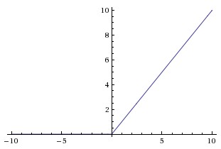
It's absurdly simple. The sigmoid function was, for a long time, the default activation function for neural networks. ReLU is certainly more common in deep learning nets, I think because they require less computational effort.
The model is 'fit' - by which I mean an optimal set weights are found - via backpropagation and stochastic gradient descent. (Reminder: We looked at gradient descent in an earlier post, Real-time learning in data streams using stochastic gradient descent, and neural net backpropagation in How neural net autoencoders can automatically abstract visual features from handwriting). A neat benefit of training with gradient descent is that it's super-easy to resume training if new data appears. These things are expensive to train, but once it is then we can cheaply continue to update it forever.
Despite the small sample size and small network (9 layers is pretty small for deep learning), the computation required to train this CNN is significant. Across all layers, there's 8,446,466 weight and bias parameters to learn! On a Google Compute Engine instance with 16 vCPUs, 100 epochs took around 5 hours (cost: ~AUD$5), ultimately achieving a train accuracy of 98.2%. Neural nets are notorious for overfitting and, unsurprisingly, the test results are substantially lower (~88%).
TensorFlow's TensorBoard gives us lots of charts and diagnostics, including:

What has it learned?
CNNs are very black-boxy and it’s hard to get any kind of understanding of what they have learned. This is because there are so many layers, and the deeper layers - which are supposedly the ones that learn the “higher-level” features - are so far removed from the input images.
We can get a feeling for what the first convolution layer is doing. I don’t see much point in plotting the 32 filters (they’re only 3x3x3), but we can feed that layer an image and visualise its outputs to understand what its filters do.


What is remarkable is that the layer has learned a variety of filters which can detect edges and separate elements of the picture. Most importantly, some filters isolate the cat from the background. We haven’t had to supply any edge-detection algorithms - the CNN has learned its own. And plainly that’s a useful thing: being able to isolate the animal from the rest of the image is step one towards identifying what it is.
Here’s one more example, this time with a heat-map gradient:


Here is the crude, hacky code which I used to generate these plots:
Understanding what the deeper layers are doing is not so easy. An intriguing approach is described in this paper, where the authors use a "deconvnet" to map intermediate layers back to input pixel space.
How good is our CNN?
Sadly, it's a long way short of state-of-the-art. The winner of Kaggle's Dogs vs. Cats competition achieved 98.9% test accuracy.
How to get to 98.9%? There's a lot of effort required to eke out those extra percent. They include things like:
- Bigger networks with more layers: ResNet - the winner of the 2015 ImageNet Large Scale Visual Recognition Challenge (ILSVRC) - has 152 layers. (And if that wasn’t enough, to win they competition they used an ensemble of ResNets). Paper here.
- Pre-training: the winner of the Kaggle Dogs vs. Cats competition wrote, "My system was pre-trained on ImageNet (ILSVRC12 classification dataset) and subsequently refined on the cats and dogs data" [italics mine]. The ImageNet ILSVRC12 dataset contains 10m labelled images depicting 10k objects. Even if there aren't many cats and dogs in the pre-training data, it helps the CNN learn useful filters for distinguishing objects in images. This is sometimes called "transfer learning." (Also, it should go without saying that more training sample is always going to help).
- Larger, higher-resolution images: In this tutorial, I chose to downsize images to 64x64 to reduce computational demands. But downsizing sacrifices information; larger images have more detail and afford larger filters.
- Bagging, ensembles and using CNNs as inputs to other ML techniques: the 8th placed contestant in Kaggle's competition described some of their approaches on their blog.
But I think the results we've gotten from a fairly vanilla CNN are pretty great, especially considering how little code & effort was required. And let's put it in historical context: in 2007, computer security researchers were saying that machines would not surpass 60% accuracy at distinguishing cats from dogs "barring a major advance in machine vision" or a "major AI advance." (see Asirra: A CAPTCHA that Exploits Interest-Aligned Manual Image Categorization).
The end
That's it. I've simplified CNNs considerably because I wanted to concentrate on the intuition. For those who want more, I highly recommend the notes from Stanford CS231n: Convolutional Neural Networks for Visual Recognition. I also found An Intuitive Explanation of Convolutional Neural Networks very helpful for its illustrations of how filters work.
In the next post we'll be looking at another type of deep learning, the Long Short-Term Memory (LSTM) neural network, which specialises in learning complex sequence patterns such as we find in language or music.
[^1]: Acknowledgements: this code was based on the tflearn CIFAR-10 CNN tutorial code, which itself seems to be basically an implementation of Google's TensorFlow CNN CIFAR-10 tutorial code.